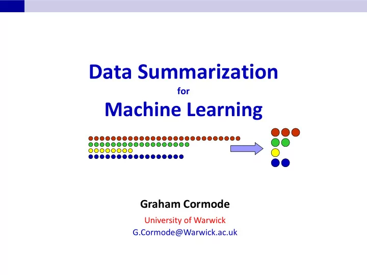
Data Summarization for Machine Learning Graham Cormode University - PowerPoint PPT Presentation
Data Summarization for Machine Learning Graham Cormode University of Warwick G.Cormode@Warwick.ac.uk The case for Big Data in one slide Big data arises in many forms: Medical data: genetic sequences, time series Activity
Data Summarization for Machine Learning Graham Cormode University of Warwick G.Cormode@Warwick.ac.uk
The case for “Big Data” in one slide “Big” data arises in many forms: – Medical data: genetic sequences, time series – Activity data: GPS location, social network activity – Business data: customer behavior tracking at fine detail – Physical Measurements: from science (physics, astronomy) Common themes: – Data is large, and growing – There are important patterns and trends in the data – We want to (efficiently) find patterns and make predictions “ Big data ” is about more than simply the volume of the data – But large datasets present a particular challenge for us! 2
Computational scalability The first (prevailing) approach: scale up the computation Many great technical ideas: – Use many cheap commodity devices – Accept and tolerate failure – Move code to data, not vice-versa – MapReduce: BSP for programmers – Break problem into many small pieces – Add layers of abstraction to build massive DBMSs and warehouses – Decide which constraints to drop: noSQL, BASE systems Scaling up comes with its disadvantages: – Expensive (hardware, equipment, energy ), still not always fast This talk is not about this approach! 3
Downsizing data A second approach to computational scalability: scale down the data! – A compact representation of a large data set – Capable of being analyzed on a single machine – What we finally want is small: human readable analysis / decisions – Necessarily gives up some accuracy: approximate answers – Often randomized (small constant probability of error) – Much relevant work: samples, histograms, wavelet transforms Complementary to the first approach: not a case of either-or Some drawbacks: – Not a general purpose approach: need to fit the problem – Some computations don’t allow any useful summary 4
Outline for the talk Part 1: Few examples of compact summaries (no proofs) – Sketches: Bloom filter, Count-Min, AMS – Sampling: count distinct, distinct sampling – Summaries for more complex objects: graphs and matrices Part 2: Some recent work on summaries for ML tasks – Distributed construction of Bayesian models – Approximate constrained regression via sketching 5
Summary Construction A ‘summary’ is a small data structure, constructed incrementally – Usually giving approximate, randomized answers to queries Key methods for summaries: – Create an empty summary – Update with one new tuple: streaming processing – Merge summaries together: distributed processing (eg MapR) – Query: may tolerate some approximation (parameterized by ε ) Several important cost metrics (as function of ε , n): – Size of summary, time cost of each operation 6
Bloom Filters Bloom filters [Bloom 1970] compactly encode set membership – E.g. store a list of many long URLs compactly – k hash functions map items to m-bit vector k times – Update: Set all k entries to 1 to indicate item is present – Query: Can lookup items, store set of size n in O(n) bits Analysis: choose k and size m to obtain small false positive prob item 1 1 1 Duplicate insertions do not change Bloom filters Can be merge by OR-ing vectors (of same size) 7
Bloom Filters Applications Bloom Filters widely used in “big data” applications – Many problems require storing a large set of items Can generalize to allow deletions – Swap bits for counters: increment on insert, decrement on delete – If representing sets, small counters suffice: 4 bits per counter – If representing multisets, obtain (counting) sketches Bloom Filters are an active research area – Several papers on topic in every networking conference… item 1 1 1 8
Count-Min Sketch Count Min sketch [C, Muthukrishnan 04] encodes item counts – Allows estimation of frequencies (e.g. for selectivity estimation) – Some similarities in appearance to Bloom filters Model input data as a vector x of dimension U – Create a small summary as an array of w d in size – Use d hash function to map vector entries to [1..w] W Array: d CM[i,j] 9
Count-Min Sketch Structure +c h 1 (j) d rows +c j,+c +c h d (j) +c w = 2/ e Update: each entry in vector x is mapped to one bucket per row. Merge two sketches by entry-wise summation Query: estimate x[j] by taking min k CM[k,h k (j)] – Guarantees error less than e ‖x‖ 1 in size O(1/ e ) – Probability of more error reduced by adding more rows 10
Generalization: Sketch Structures Sketch is a class of summary that is a linear transform of input – Sketch(x) = Sx for some matrix S – Hence, Sketch( x + y) = Sketch(x) + Sketch(y) – Trivial to update and merge Often describe S in terms of hash functions – S must have compact description to be worthwhile – If hash functions are simple, sketch is fast Analysis relies on properties of the hash functions – Seek “limited independence” to limit space usage – Proofs usually study the expectation and variance of the estimates 11
Sketching for Euclidean norm AMS sketch presented in [Alon Matias Szegedy 96] 2 – Allows estimation of F 2 (second frequency moment) aka ‖x‖ 2 – Leads to estimation of (self) join sizes, inner products – Used at the heart of many streaming and non-streaming applications: achieves dimensionality reduction (‘Johnson -Lindenstrauss lemma’) Here, describe the related CountSketch by generalizing CM sketch – Use extra hash functions g 1 ...g d {1...U} {+1,-1} – Now, given update (j,+c), set CM[k,h k (j)] += c*g k (j) Estimate squared Euclidean norm (F 2 ) = median k i CM[k,i] 2 – Intuition: g k hash values cause ‘cross - terms’ to cancel out, on average +c*g 1 (j) – The analysis formalizes this intuition h 1 (j) +c*g 2 (j) j,+c – median reduces chance of large error +c*g 3 (j) h d (j) 12 +c*g 4 (j)
L 0 Sampling L 0 sampling: sample item i with prob (1± e ) f i 0 /F 0 (# distinct items) – i.e., sample (near) uniformly from items with non-zero frequency – Challenging when frequencies can increase and decrease General approach: [Frahling, Indyk, Sohler 05, C., Muthu, Rozenbaum 05] – Sub-sample all items (present or not) with probability p – Generate a sub-sampled vector of frequencies f p – Feed f p to a k-sparse recovery data structure (sketch summary) Allows reconstruction of f p if F 0 < k, uses space O(k) – If f p is k-sparse, sample from reconstructed vector – Repeat in parallel for exponentially shrinking values of p 13
Sampling Process p=1/U k-sparse recovery p=1 Exponential set of probabilities, p=1, ½, ¼, 1/8, 1/16… 1/U – Want there to be a level where k-sparse recovery will succeed Sub-sketch that can decode a vector if it has few non-zeros – At level p, expected number of items selected S is pF 0 – Pick level p so that k/3 < pF 0 2k/3 Analysis: this is very likely to succeed and sample correctly 14
Graph Sketching Given L 0 sampler, use to sketch (undirected) graph properties Connectivity: find the connected components of the graph Basic alg: repeatedly contract edges between components – Implement: Use L 0 sampling to get edges from vector of adjacencies – One sketch for the adjacency list for each node Problem: as components grow, sampling edges from components most likely to produce internal links 15
Graph Sketching Idea: use clever encoding of edges [ Ahn, Guha, McGregor 12] Encode edge (i,j) as ((i,j),+1) for node i<j, as ((i,j),-1) for node j>i When node i and node j get merged, sum their L 0 sketches – Contribution of edge (i,j) exactly cancels out + i = j – Only non-internal edges remain in the L 0 sketches Use independent sketches for each iteration of the algorithm – Only need O(log n) rounds with high probability Result: O(poly-log n) space per node for connected components 16
Matrix Sketching Given matrices A, B, want to approximate matrix product AB – Measure the normed error of approximation C: ǁ AB – C ǁ Main results for the Frobenius (entrywise) norm ǁ ǁ F – ǁCǁ F = ( i,j C i,j 2 ) ½ – Results rely on sketches, so this entrywise norm is most natural 17
Direct Application of Sketches Build AMS sketch of each row of A (A i ), each column of B (B j ) Estimate C i,j by estimating inner product of A i with B j – Absolute error in estimate is e ǁA i ǁ 2 ǁB j ǁ 2 (whp) – Sum over all entries in matrix, Frobenius error is e ǁAǁ F ǁBǁ F Outline formalized & improved by Clarkson & Woodruff [09,13] – Improve running time to linear in number of non-zeros in A,B 18
More Linear Algebra Matrix multiplication improvement: use more powerful hash fns – Obtain a single accurate estimate with high probability Linear regression given matrix A and vector b: find x R d to (approximately) solve min x ǁ Ax – b ǁ – Approach : solve the minimization in “sketch space” – From a summary of size O(d 2 / e ) [independent of rows of A] Frequent directions: approximate matrix-vector product [Ghashami, Liberty, Phillips, Woodruff 15] – Use the SVD to (incrementally) summarize matrices The relevant sketches can be built quickly: proportional to the number of nonzeros in the matrices (input sparsity) – Survey: Sketching as a tool for linear algebra [Woodruff 14] 19
Recommend
More recommend
Explore More Topics
Stay informed with curated content and fresh updates.
