Data Structures Fibonacci Heaps, Amortized Analysis Algorithm Theory - PowerPoint PPT Presentation
Chapter 4 Data Structures Fibonacci Heaps, Amortized Analysis Algorithm Theory WS 2012/13 Fabian Kuhn Fibonacci Heaps Lacy merge variant of binomial heaps: Do not merge trees as long as possible Structure: A Fibonacci heap consists
Chapter 4 Data Structures Fibonacci Heaps, Amortized Analysis Algorithm Theory WS 2012/13 Fabian Kuhn
Fibonacci Heaps Lacy ‐ merge variant of binomial heaps: • Do not merge trees as long as possible… Structure: A Fibonacci heap � consists of a collection of trees satisfying the min ‐ heap property. Variables: • �. ��� : root of the tree containing the (a) minimum key • �. �������� : circular, doubly linked, unordered list containing the roots of all trees • �. ���� : number of nodes currently in � Algorithm Theory, WS 2012/13 Fabian Kuhn 2
Trees in Fibonacci Heaps Structure of a single node � : parent right left key degree child mark • �. ����� : points to circular, doubly linked and unordered list of the children of � • �. ���� , �. ����� : pointers to siblings (in doubly linked list) • �. ���� : will be used later… Advantages of circular, doubly linked lists: • Deleting an element takes constant time • Concatenating two lists takes constant time Algorithm Theory, WS 2012/13 Fabian Kuhn 3
Example Figure: Cormen et al., Introduction to Algorithms Algorithm Theory, WS 2012/13 Fabian Kuhn 4
Simple (Lazy) Operations Initialize ‐ Heap � : • �. �������� ≔ �. ��� ≔ ���� Merge heaps � and �′ : • concatenate root lists • update �. ��� Insert element � into � : • create new one ‐ node tree containing � H′ • merge heaps � and �′ Get minimum element of � : • return �. ��� Algorithm Theory, WS 2012/13 Fabian Kuhn 5
Operation Delete ‐ Min Delete the node with minimum key from � and return its element: � ≔ �. ���; 1. if �. ���� � 0 then 2. remove �. ��� from �. �������� ; 3. add �. ���. ����� (list) to �. �������� 4. �. ������������� ; 5. // Repeatedly merge nodes with equal degree in the root list // until degrees of nodes in the root list are distinct. // Determine the element with minimum key return � 6. Algorithm Theory, WS 2012/13 Fabian Kuhn 6
Rank and Maximum Degree Ranks of nodes, trees, heap: Node � : • ������� : degree of � Tree � : • ���� � : rank (degree) of root node of � Heap � : • ������� : maximum degree of any node in � Assumption ( � : number of nodes in � ): ���� � � ���� – for a known function ���� Algorithm Theory, WS 2012/13 Fabian Kuhn 7
Merging Two Trees Given: Heap ‐ ordered trees � , �′ with ���� � � ������ � � • Assume: min ‐ key of � � min ‐ key of �′ Operation ������, � � � : ���� � �′ • Removes tree �′ from root list and adds � � to child list of � • ���� � ≔ ���� � � 1 � • � � . ���� ≔ ����� �′ Algorithm Theory, WS 2012/13 Fabian Kuhn 8
Consolidation of Root List Array � pointing to find roots with the same rank: 0 1 2 ���� Consolidate: Time: for � ≔ 0 to ���� do � � ≔ null ; 1. ��|�. �������� �� � ��|�. �������� �� � while �. �������� � null do 2. � ≔ “delete and return first element of �. �������� ” 3. while � ���� � � null do 4. � � ≔ � ���� � ; 5. � ���� � ≔ ����; 6. � ≔ ������, � � � 7. � ���� � ≔ � 8. Create new �. �������� and �. ��� 9. Algorithm Theory, WS 2012/13 Fabian Kuhn 9
Operation Decrease ‐ Key Decrease ‐ Key ��, �� : (decrease key of node � to new value � ) if � � �. ��� then return ; 1. �. ��� ≔ �; update �. ��� ; 2. if � ∈ �. �������� ∨ � � �. ������. ��� then return 3. 4. repeat ������ ≔ �. ������; 5. �. ��� � ; 6. � ≔ ������; 7. until � �. ���� ∨ � ∈ �. �������� ; 8. if � ∉ �. �������� then �. ���� ≔ ���� ; 9. Algorithm Theory, WS 2012/13 Fabian Kuhn 10
Operation Cut( ) Operation �. ������ : • Cuts � ’s sub ‐ tree from its parent and adds � to rootlist if � ∉ �. �������� then 1. // cut the link between � and its parent 2. ���� �. ������ ≔ ���� �. ������ � 1 ; 3. remove � from �. ������. ����� (list) 4. �. ������ ≔ null ; 5. add � to �. �������� 6. � 1 2 15 1 3 2 15 � 19 7 ������ ������ 13 8 13 8 25 3 25 19 7 31 31 Algorithm Theory, WS 2012/13 Fabian Kuhn 11
Decrease ‐ Key Example • Green nodes are marked 5 1 2 15 17 9 14 13 8 20 25 3 19 7 � 31 12 18 Decrease ‐ Key ��, �� 22 5 18 9 1 2 15 17 14 22 12 13 8 20 25 3 19 7 31 Algorithm Theory, WS 2012/13 Fabian Kuhn 12
Fibonacci Heap Marks History of a node � : � is being linked to a node �. ���� ≔ ����� a child of � is cut �. ���� ≔ ���� a second child of � is cut �. ������ • Hence, the boolean value �. ���� indicates whether node � has lost a child since the last time � was made the child of another node. Algorithm Theory, WS 2012/13 Fabian Kuhn 13
Cost of Delete ‐ Min & Decrease ‐ Key Delete ‐ Min: Delete min. root � and add �. ����� to �. �������� 1. time: � 1 Consolidate �. �������� 2. time: � length of �. �������� � ���� Step 2 can potentially be linear in � (size of � ) • Decrease ‐ Key (at node � ): If new key � parent key, cut sub ‐ tree of node � 1. time: ��1� 2. Cascading cuts up the tree as long as nodes are marked time: ��number of consecutive marked nodes� Step 2 can potentially be linear in � • Exercises: Both operations can take ���� time in the worst case! ���� Algorithm Theory, WS 2012/13 Fabian Kuhn 14
Cost of Delete ‐ Min & Decrease ‐ Key • Cost of delete ‐ min and decrease ‐ key can be Θ��� … – Seems a large price to pay to get insert and merge in ��1� time • Maybe, the operations are efficient most of the time? – It seems to require a lot of operations to get a long rootlist and thus, an expensive consolidate operation – In each decrease ‐ key operation, at most one node gets marked: We need a lot of decrease ‐ key operations to get an expensive decrease ‐ key operation • Can we show that the average cost per operation is small? • We can requires amortized analysis Algorithm Theory, WS 2012/13 Fabian Kuhn 15
Amortization • Consider sequence � � , � � , … , � � of � operations (typically performed on some data structure � ) • � � : execution time of operation � � • � ≔ � � � � � � ⋯ � � � : total execution time • The execution time of a single operation might vary within a large range (e.g., � � ∈ �1, � � � ) • The worst case overall execution time might still be small average execution time per operation might be small in the worst case, even if single operations can be expensive Algorithm Theory, WS 2012/13 Fabian Kuhn 16
Analysis of Algorithms • Best case • Worst case • Average case • Amortized worst case What it the average cost of an operation in a worst case sequence of operations? Algorithm Theory, WS 2012/13 Fabian Kuhn 17
Example: Binary Counter Incrementing a binary counter: determine the bit flip cost: Operation Counter Value Cost 00000 1 0000 1 1 2 000 10 2 3 0001 1 1 4 00 100 3 5 0010 1 1 6 001 10 2 7 0011 1 1 8 0 1000 4 9 0100 1 1 10 010 10 2 11 0101 1 1 12 01 100 3 13 0110 1 1 Algorithm Theory, WS 2012/13 Fabian Kuhn 18
Accounting Method Observation: • Each increment flips exactly one 0 into a 1 00100�1111 ⟹ 00100�0000 Idea: • Have a bank account (with initial amount 0) • Paying � to the bank account costs � • Take “money” from account to pay for expensive operations Applied to binary counter: • Flip from 0 to 1: pay 1 to bank account (cost: 2) • Flip from 1 to 0: take 1 from bank account (cost: 0) • Amount on bank account = number of ones We always have enough “money” to pay! Algorithm Theory, WS 2012/13 Fabian Kuhn 19
Accounting Method Op. Counter Cost To Bank From Bank Net Cost Credit 0 0 0 0 0 1 0 0 0 0 1 1 2 0 0 0 1 0 2 3 0 0 0 1 1 1 4 0 0 1 0 0 3 5 0 0 1 0 1 1 6 0 0 1 1 0 2 7 0 0 1 1 1 1 8 0 1 0 0 0 4 9 0 1 0 0 1 1 10 0 1 0 1 0 2 Algorithm Theory, WS 2012/13 Fabian Kuhn 20
Recommend
More recommend
Explore More Topics
Stay informed with curated content and fresh updates.
