Data Locality in MapReduce Loris Marchal 1 Olivier Beaumont 2 1: - PowerPoint PPT Presentation
Data Locality in MapReduce Loris Marchal 1 Olivier Beaumont 2 1: CNRS and ENS Lyon, France. 2: INRIA Bordeaux Sud-Ouest, France. New Challenges in Scheduling Theory March 2016 1/ 29 MapReduce basics Well known framework for
Data Locality in MapReduce Loris Marchal 1 Olivier Beaumont 2 1: CNRS and ENS Lyon, France. 2: INRIA Bordeaux Sud-Ouest, France. New Challenges in Scheduling Theory — March 2016 1/ 29
MapReduce basics ◮ Well known framework for data-processing on parallel clusters ◮ Popularized by Google, open source implementation: Apache Hadoop ◮ Breaks computation into small tasks, distributed on the processors ◮ Dynamic scheduler: handle failures and processor heterogeneity ◮ Centralized scheduler launches all tasks ◮ Users only have to write code for two functions: ◮ Map: filters the data, produces intermediate results ◮ Reduce: summarizes the information ◮ Large data files split into chunks that are scattered on the platform (e.g. using HDFS for Hadoop) ◮ Goal: process computation near the data, avoid large data transfers 2/ 29
MapReduce example Textbook example: WordCount (count #occurrences of words in a text) 1. Text split in chunks scattered on local disks 2. Map: compute #occurrences of words in each chunk, produces results as < word,#occurrences > pairs 3. Sort and Shuffle: gather all pairs with same word on a single processor 4. Reduce: merges results for single word (sum #occurrences) 3/ 29
Other usages of MapReduce ◮ Several phases of Map and Reduce (tightly coupled applications) ◮ Only Map phase (independent tasks, divisible load scheduling) 4/ 29
MapReduce locality Potential data transfer sources: ◮ Sort and Shuffle: data exchange between all processors ◮ Depends on the applications (size and number of < key,value > pairs) ◮ Map task allocation: when a Map slot is available on a processor ◮ choose a local chunk if any ◮ otherwise choose any unprocessed chunk and transfer data Replication during initial data distributions: ◮ To improve (data locality) and fault tolerance ◮ Optional, basic setting: 3 replicas ◮ first, chunk placed on a disk ◮ one copy sent to another disk of the same rack (local communication) ◮ one copy sent to another rack 5/ 29
Objective of this study Analyze the data locality of the Map phase: 1. estimate the volume of communication 2. estimate the load imbalance without communication Using a simple model, to provide good estimates and measure the influence of key parameters: ◮ Replication factor ◮ Number of tasks and processors ◮ Task heterogeneity (to come) Disclaimer: work in progress Comments/contributions welcome! 6/ 29
Outline Introduction & motivation Related work Volume of communication of the Map phase Load imbalance without communication Conclusion 7/ 29
Outline Introduction & motivation Related work Volume of communication of the Map phase Load imbalance without communication Conclusion 8/ 29
Related work 1/2 MapReduce locality: ◮ Improvement Shuffle phase ◮ Few studies on the locality for the Map phase (mostly experimental) Balls-into-bins: ◮ Random allocation of n balls in p bins: ◮ For n = p , maximum load of log n / log log n ◮ Estimation of maximum load with high probability for n ≥ p [Raab & Steeger 2013] ◮ Choosing the least loaded among r candidates improves a lot ◮ “Power of two choices” [Mitzenmacher 2001] ◮ Maximum load n / p + O (log log p ) [Berenbrick et al. 2000] ◮ Adaptation for weighted balls [Berenbrick et al. 2008] 9/ 29
Related work 1/2 MapReduce locality: ◮ Improvement Shuffle phase ◮ Few studies on the locality for the Map phase (mostly experimental) Balls-into-bins: ◮ Random allocation of n balls in p bins: ◮ For n = p , maximum load of log n / log log n ◮ Estimation of maximum load with high probability for n ≥ p [Raab & Steeger 2013] ◮ Choosing the least loaded among r candidates improves a lot ◮ “Power of two choices” [Mitzenmacher 2001] ◮ Maximum load n / p + O (log log p ) [Berenbrick et al. 2000] ◮ Adaptation for weighted balls [Berenbrick et al. 2008] 9/ 29
Related work 2/2 Work-stealing: ◮ Independent tasks or tasks with precedence ◮ Steal part of a victim’s task queue in time 1 ◮ Distributed process (steal operations may fail) ◮ Bound on makespan using potential function [Tchiboukdjian, Gast & Trystram 2012] 10/ 29
Outline Introduction & motivation Related work Volume of communication of the Map phase Load imbalance without communication Conclusion 11/ 29
Problem statement – MapReduce model Data distribution: ◮ p processors, each with its own data storage (disk) ◮ n tasks (or chunks) ◮ r copies of each chunk distributed uniformly at random Allocation strategy: ◮ whenever a processor is idle: ◮ allocate a local task is possible ◮ otherwise, allocate a random task, copy the data chunk ◮ invalidate all other replicas of the chosen chunk Cost model: ◮ Uniform chunk size (parameter of MapReduce) ◮ Uniform task durations Question: ◮ Total volume of communication (in chunk number) 12/ 29
Problem statement – MapReduce model Data distribution: ◮ p processors, each with its own data storage (disk) ◮ n tasks (or chunks) ◮ r copies of each chunk distributed uniformly at random Allocation strategy: ◮ whenever a processor is idle: ◮ allocate a local task is possible ◮ otherwise, allocate a random task, copy the data chunk ◮ invalidate all other replicas of the chosen chunk Cost model: ◮ Uniform chunk size (parameter of MapReduce) ◮ Uniform task durations Question: ◮ Total volume of communication (in chunk number) 12/ 29
Problem statement – MapReduce model Data distribution: ◮ p processors, each with its own data storage (disk) ◮ n tasks (or chunks) ◮ r copies of each chunk distributed uniformly at random Allocation strategy: ◮ whenever a processor is idle: ◮ allocate a local task is possible ◮ otherwise, allocate a random task, copy the data chunk ◮ invalidate all other replicas of the chosen chunk Cost model: ◮ Uniform chunk size (parameter of MapReduce) ◮ Uniform task durations Question: ◮ Total volume of communication (in chunk number) 12/ 29
Problem statement – MapReduce model Data distribution: ◮ p processors, each with its own data storage (disk) ◮ n tasks (or chunks) ◮ r copies of each chunk distributed uniformly at random Allocation strategy: ◮ whenever a processor is idle: ◮ allocate a local task is possible ◮ otherwise, allocate a random task, copy the data chunk ◮ invalidate all other replicas of the chosen chunk Cost model: ◮ Uniform chunk size (parameter of MapReduce) ◮ Uniform task durations Question: ◮ Total volume of communication (in chunk number) 12/ 29
Simple solution ◮ Consider the system after k chunks have been allocated ◮ A processor i requests a new task ◮ Assumption: the remaining r ( n − k ) replicas are uniformly distributed ◮ Probability that none of them reach i : � r ( n − k ) � 1 − 1 = 1 − r ( n − k ) � 1 � � 1 � = e − r ( n − k ) / p + o p k = + o p p p p ◮ Fraction of non-local chunks: f = 1 p k = p � rn (1 − e − rn / p ) n k 13/ 29
Simple solution - simulations p=1000 processors, m=10.000 tasks 0 . 2 0 . 18 0 . 16 fraction of non local tasks 0 . 14 0 . 12 MapReduce simulations 0 . 1 1-f 0 . 08 0 . 06 0 . 04 0 . 02 0 1 2 3 4 5 6 replication factor ◮ Largely underestimates non-local tasks without replication ( r = 1) ◮ Average accuracy with replication ( r > 1) 14/ 29
Simple solution - questioning the assumption Remaining chunks without replication: (100 processors, 1000 tasks) initial distribution (10 chunks/procs on average) Non uniform distribution after some time � 15/ 29
Simple solution - questioning the assumption Remaining chunks without replication: (100 processors, 1000 tasks) after 200 steps Non uniform distribution after some time � 15/ 29
Simple solution - questioning the assumption Remaining chunks without replication: (100 processors, 1000 tasks) after 400 steps Non uniform distribution after some time � 15/ 29
Simple solution - questioning the assumption Remaining chunks without replication: (100 processors, 1000 tasks) after 600 steps Non uniform distribution after some time � 15/ 29
Simple solution - questioning the assumption Remaining chunks without replication: (100 processors, 1000 tasks) after 800 steps Non uniform distribution after some time � 15/ 29
Simple solution - questioning the assumption Remaining chunks without replication: (100 processors, 1000 tasks) after 800 steps Non uniform distribution after some time � 15/ 29
Simple solution - questioning the assumption Remaining chunks with replication=3: (100 processors, 1000 tasks) initial distribution (30 chunks/procs on average) Uniform distribution for a large part of the execution? 16/ 29
Simple solution - questioning the assumption Remaining chunks with replication=3: (100 processors, 1000 tasks) after 200 steps Uniform distribution for a large part of the execution? 16/ 29
Simple solution - questioning the assumption Remaining chunks with replication=3: (100 processors, 1000 tasks) after 400 steps Uniform distribution for a large part of the execution? 16/ 29
Simple solution - questioning the assumption Remaining chunks with replication=3: (100 processors, 1000 tasks) after 600 steps Uniform distribution for a large part of the execution? 16/ 29
Recommend
More recommend
Explore More Topics
Stay informed with curated content and fresh updates.
