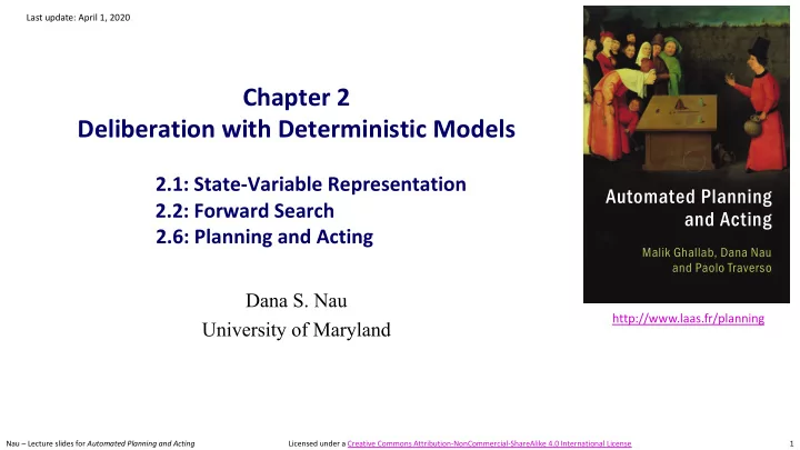
[PPT] - Chapter 2 Deliberation with Deterministic Models 2.1: PowerPoint Presentation

SLIDE 1

1 Nau – Lecture slides for Automated Planning and Acting

Automated Planning and Acting

Malik Ghallab, Dana Nau and Paolo Traverso

Last update: April 1, 2020

http://www.laas.fr/planning

Licensed under a Creative Commons Attribution-NonCommercial-ShareAlike 4.0 International License

Chapter 2 Deliberation with Deterministic Models

2.1: State-Variable Representation 2.2: Forward Search 2.6: Planning and Acting

Dana S. Nau University of Maryland

SLIDE 2

2 Nau – Lecture slides for Automated Planning and Acting

Motivation and Outline

How to model a complex environment?

▸ Generally need simplifying assumptions

Classical planning
Finite, static world, just one actor
No concurrent actions, no explicit time
Determinism, no uncertainty

▸ Sequence of states and actions ⟨s0, a1, s1, a2, s2, …⟩

Avoids many complications
Most real-world environments don’t satisfy the assumptions

⇒ Errors in prediction

OK if they’re infrequent and don’t have severe consequences

Outline 2.1 State-variable representation ▸ state variables, states, actions, plans 2.2 Forward state-space search 2.6 Incorporating planning into an actor 2.3 Heuristic functions 2.4 Backward search 2.5 Plan-space search

SLIDE 3

3 Nau – Lecture slides for Automated Planning and Acting

Domain Model

State-transition system

r classical planning domain:
Σ = (S,A,γ,cost) or (S,A,γ)

▸ S - finite set of states ▸ A - finite set of actions ▸ γ: S × A → S

prediction (or state-transition) function
partial function

▸ defined only when a is applicable in s

Domain(a) = {s ∈ S | a is applicable in s}

= {s ∈ S | γ(s,a) is defined}

Range(a) = {γ(s,a) | s ∈ Domain(a)}

▸ cost: S × A → R +

r cost: A → R +
optional; default is cost(a) ≡ 1
money, time, something else
plan:

▸ a sequence of actions π = ⟨a1, …, an⟩

π is applicable in s0 if the actions are applicable in

the order given γ(s0, a1) = s1 γ(s1, a2) = s2 … γ(sn–1, an) = sn ▸ In this case define γ(s0, π) = sn

Classical planning problem:

▸ P = (Σ, s0, Sg) ▸ planning domain, initial state, set of goal states

Solution for P:

▸ a plan π such that that γ(s0,π) ∈ Sg

SLIDE 4

4 Nau – Lecture slides for Automated Planning and Acting

If S and A are small enough

▸ Give each state and action a name ▸ For each s and a, store γ(s,a) in a lookup table

In larger domains, don’t represent all states

explicitly ▸ Language for describing properties of states ▸ Language for describing how each action changes those properties ▸ Start with initial state ▸ Use actions to produce other states

loc1 loc3 loc2 loc6 loc5 loc4 loc7 loc8 loc0

x y

4 3 2 1 1 2 3 4 5 6 loc9

Representing Σ

a1′

…

s0 a1 s1 = γ(s0,a1) s1′ = γ(s0,a1′)

…

SLIDE 5

5 Nau – Lecture slides for Automated Planning and Acting

Domain-Specific Representation

Made to order for a specific environment
State: arbitrary data structure
Action: (head, preconditions, effects, cost)

▸ head: name and parameter list

Get actions by instantiating the parameters

▸ preconditions:

Computational tests to predict whether an action can be performed
Should be necessary/sufficient for the action to run without error

▸ effects:

Procedures that modify the current state

▸ cost: procedure that returns a number

Can be omitted, default is cost ≡ 1

SLIDE 6

6 Nau – Lecture slides for Automated Planning and Acting

Example

Drilling holes in a metal workpiece

▸ A state

annotated geometric model of the workpiece
capabilities and status of

drilling machine and drill bit ▸ Several actions

put workpiece onto the drilling machine
clamp it
load a drill bit
drill
Name and parameters:

▸ drill-hole(machine, drill-bit, workpiece, geometry, machining-tolerances)

Preconditions

▸ Capabilities: can the machine and drill bit produce a hole with the desired geometry and machining tolerances? ▸ Current state: Is the drill bit installed? Is the workpiece clamped onto the table? Etc.

Effects

▸ annotated geometric model of modified workpiece

Cost

▸ estimate of time or monetary cost

SLIDE 7

7 Nau – Lecture slides for Automated Planning and Acting

Discussion

Advantage of domain-specific representation:

▸ use whatever works best for that particular domain

Disadvantage:

▸ for each new domain, need new representation and deliberation algorithms

Alternative: domain-independent representation

▸ Try to create a “standard format” that can be used for many different planning domains ▸ Deliberation algorithms that work for anything in this format

State-variable representation

▸ Simple formats for describing states and actions ▸ Limited representational capability

But easy to compute, easy to reason

about ▸ Domain-independent search algorithms and heuristic functions that can be used in all state-variable planning problems

SLIDE 8

8 Nau – Lecture slides for Automated Planning and Acting

State-Variable Representation

E: environment that we want to represent
B: set of symbols called objects

▸ names for objects in E, mathematical constants, …

Example

▸ B = Robots ∪ Containers ∪ Locs ∪ {nil}

Robots = {r1}
Containers = {c1, c2}
Locs = {d1, d2, d3}
B only needs to include objects that matter at the current level of abstraction
Can omit lots of details

▸ physical characteristics of robots, containers, loading docks, roads, …

d2 d1 d3 r1 c1 c2

SLIDE 9

9 Nau – Lecture slides for Automated Planning and Acting

Properties of Objects

Define ways to represent properties of objects

▸ Two kinds of properties: rigid and varying

Rigid property: stays the same in every state

▸ Two equivalent notations:

A mathematical relation

adjacent = {(d1,d2), (d2,d1), (d1,d3), (d3,d1)}

A set of ground atoms

adjacent(d1,d2), adjacent(d2,d1), adjacent(d1,d3), adjacent(d3,d1)

Terminology from first-order logic:

▸ ground: fully instantiated, no variable symbols ▸ atom ≡ atomic formula ≡ positive literal ≡ predicate symbol with list of arguments ▸ negative literal ≡ negated atom ≡ atom with a negation sign in front of it

d2 d1 d3 r1 c1 c2

SLIDE 10

10 Nau – Lecture slides for Automated Planning and Acting

Varying Properties

Varying property (or fluent): may differ in different states

▸ Represent it using a state variable that we can assign a value to

Set of state variables

X = {loc(r1), loc(c1), loc(c2), cargo(r1)}

Each state variable x ∈ X has a range

= {all values that can be assigned to x} ▸ Range(loc(r1)) = Locs ▸ Range(loc(c1)) = Range(loc(c2)) = Robots ∪ Locs ▸ Range(cargo(r1)) = Containers ∪ {nil}

Instead of “domain”, to avoid confusion with planning domains d2 d1 d3 r1 c1 c2

SLIDE 11

11 Nau – Lecture slides for Automated Planning and Acting

States as Functions

Represent each state as a variable-assignment function

▸ Function that maps each x ∈ X to a value in Range(x) s1(loc(r1)) = d1, s1(cargo(r1)) = nil, s1(loc(c1)) = d1, s1(loc(c2)) = d2

Mathematically, a function is a set of ordered pairs

s1 = {(loc(r1), d1), (cargo(r1), nil), (loc(c1), d1) , (loc(c2), d2)}

Write it as a set of ground positive literals (or ground atoms):

s1 = {loc(r1)=d1, cargo(r1)=nil, loc(c1)=d1, loc(c2)=d2}

d2 d1 d3 r1 c1 c2

SLIDE 12

12 Nau – Lecture slides for Automated Planning and Acting

Action Templates

Action template: a parameterized set of actions

α = (head(α), pre(α), eff(α), cost(α))

head(α): name, parameters

Each parameter has a range ⊆ B

pre(α): precondition literals

rel(t1,…,tk), var(t1,…,tk) = t0, ¬ rel(t1,…,tk), ¬ var(t1,…,tk) = t0 ▸ Each ti is a parameter or an element of B

eff(α): effect literals

var(t1,…,tk) ← t0

cost(α): a number

▸ Optional, default is 1 move(r,l,m) pre: loc(r)=l, adjacent(l,m) eff: loc(r) ← m take(r,l,c) pre: cargo(r)=nil, loc(r)=l, loc(c)=l eff: cargo(r) ← c, loc(c) ← r put(r,l,c) pre: loc(r)=l, loc(c)=r eff: cargo(r) ← nil, loc(c) ← l Range(r) = Robots = {r1} Range(l) = Range(m) = Locs = {d1,d2,d3} Range(c) = Containers = {c1,c2}

d2 d1 d3 r1 c1 c2

SLIDE 13

13 Nau – Lecture slides for Automated Planning and Acting

Actions

A = set of action templates

move(r,l,m) pre: loc(r)=l, adjacent(l, m) eff: loc(r) ← m take(r,l,c) pre: cargo(r)=nil, loc(r)=l, loc(c)=l eff: cargo(r) ← c, loc(c) ← r put(r,l,c) pre: loc(r)=l, loc(c)=r eff: cargo(r) ← nil, loc(c) ← l Range(r) = Robots = {r1} Range(l) = Range(m) = Locs = {d1,d2,d3} Range(c) = Containers = {c1,c2}

Action: ground instance of an α ∈ A

▸ replace each parameter with something in its range

A = {all actions we can get from A}

= {all ground instances of members of A} move(r1,d1,d2) pre: loc(r1)=d1, adjacent(d1,d2) eff: loc(r1) ← d2

d2 d1 d3 r1 c1 c2

SLIDE 14

14 Nau – Lecture slides for Automated Planning and Acting

Actions

A = set of action templates

move(r,l,m) pre: loc(r)=l, adjacent(l, m) eff: loc(r) ← m take(r,l,c) pre: cargo(r)=nil, loc(r)=l, loc(c)=l eff: cargo(r) ← c, loc(c) ← r put(r,l,c) pre: loc(r)=l, loc(c)=r eff: cargo(r) ← nil, loc(c) ← l Range(r) = Robots = {r1} Range(l) = Range(m) = Locs = {d1,d2,d3} Range(c) = Containers = {c1,c2}

Action: ground instance of an α ∈ A

▸ replace each parameter with something in its range

A = {all actions we can get from A}

= {all ground instances of members of A} Poll: Let A = {the action templates on this page}. How many move actions in A? 1: 1 2: 2 3: 3 4: 4 5: 6 6: 9 7: something else

SLIDE 15

15 Nau – Lecture slides for Automated Planning and Acting

Applicability

a is applicable in s if

▸ for every positive literal l ∈ pre(a), l ∈ s or l is in one of the rigid relations ▸ for every negative literal ¬l ∈ pre(a), l ∉ s and l isn’t in any of the rigid relations

Rigid relation

adjacent = {(d1,d2), (d2,d1), (d1,d3), (d3,d1)}

State

s1 = {loc(r1)=d1, cargo(r1)=nil, loc(c1)=d1}

Action template

move(r,l,m) pre: loc(r)=l, adjacent(l, m) eff: loc(r) ← m Range(r) = Robots Range(l) = Range(m) = Locs

Applicable:

move(r1,d1,d2) pre: loc(r1)=d1, adjacent(d1,d2) eff: loc(r1) ← d2

Not applicable:

move(r1,d2,d1) pre: loc(r1)=d2, adjacent(d2,d1) eff: loc(r1) ← d1 Poll: In s1, how many applicable move actions?

1. 1
5. 5
2. 2
6. 6
3. 3
7. 7
4. 4
8. other

d2 d1 d3 r1 c1 c2

SLIDE 16

16 Nau – Lecture slides for Automated Planning and Acting

Computing γ

If a is applicable in s:

▸ γ(s,a) = {(x,w) | “x ← w” is in eff(a)} ∪ {(x,w) ∈ s | x isn’t the target of anything in eff(a)}

s2 = {loc(r1)=d2, cargo(r1)=nil, loc(c1)=d1, loc(c2)=d2}
take(r1,d2,c2)

pre: cargo(r1)=nil, loc(r1)=d2, loc(c2)=d2 eff: cargo(r1) ← c2, loc(c2) ← r1

γ(s2, take(r1,d2,c2)) =

{loc(r1)=d2, cargo(r1)=c2, loc(c1)=d1, loc(c2)=r1}

d2 d1 d3 c1 r1 c2 d2 d1 d3 c1 r1 c2

SLIDE 17

17 Nau – Lecture slides for Automated Planning and Acting

State-Variable Planning Domain

Let

B = finite set of objects R = finite set of rigid relations over B X = finite set of state variables

for every state variable x, Range(x) ⊆ B

S = state space over X = {all variable-assignment functions that have sensible interpretations} A = finite set of action templates

for every parameter y, Range(y) ⊆ B

A = {all ground instances of action templates in A} γ(s,a) = {(x,w) | eff(a) contains the effect x ← w} ∪{(x,w)∈s | x isn’t the target of any effect in eff(a)}

Then Σ = (S,A,γ) is a state-variable planning domain

SLIDE 18

18 Nau – Lecture slides for Automated Planning and Acting

d2 d1 d3 c1 r1 c2

Interpretations

Let s be a variable-assignment function

▸ s is a state only if the values make sense in the environment we’re trying to represent

relation to model theory
Can loc(c1)=r1 if cargo(r1)=nil?

▸ Not in our intended interpretation

Mapping of symbols to what they represent
Can both loc(c1)=r1 and loc(c2)=r1?

▸ In our intended interpretation, can a robot carry more than one object at a time?

How to enforce the intended interpretation?
Explicitly

▸ Mathematical axioms ▸ Integrity constraints

Implicitly

▸ Write an initial state s0 that satisfies the interpretation ▸ Write the actions in such a way that whenever s satisfies the interpretation, γ(s,a) will too s0 = {loc(r1)=d2, cargo(r1)=nil , loc(c1)=d1 , loc(c2)=d2} a3

…

s0 a2 s2 = γ(s0,a2) s3 = γ(s0,a3)

… …

a1 s1 = γ(s0,a1)

SLIDE 19

19 Nau – Lecture slides for Automated Planning and Acting

Plans

Plan: sequence of actions π = áa1,a2,…,anñ

▸ cost(π) = ∑i cost(ai)

π is applicable in s0 if the actions can be applied in the order given, i.e., there

are states s1, s2, …, sn such that g (s0,a1) = s1, g (s1,a2) = s2, …, g (sn–1,an) = sn ▸ If so, then g (s0, π) = sn

π = ámove(r1,d3,d1), take(r1,d1,c1), move(r1,d1,d3)ñ
cost(π) = 3

s3 = {loc(r1)=d3, cargo(r1)=nil, loc(c1)=d1, loc(c2)=d2} γ(s3,π) = {loc(r1)=d3, cargo(r1)=c1, loc(c1)=r1, loc(c2)=d2}

d2 d1 d3 c1 r1 c2 d2 d1 d3 r1 c2 c1

SLIDE 20

20 Nau – Lecture slides for Automated Planning and Acting

State Space

Directed graph

▸ Nodes = states of the world ▸ Directed edges: g

If π = áa1, a2, …, anñ is applicable in s0 ,

it produces a path ás0, s1, s2, …, snñ g (s0,a1) = s1, g (s1,a2) = s2, …, g (sn–1,an) = sn

d2 d1 d3 c1 r1 c2 d2 d1 d3 c1 r1 c2 d2 d1 d3 c1 r1 c2

move(r1,d1,d2) take(r1,d1,c2) move(r1,d2,d1) put(r1,d1,c2)

d2 d1 d3 c1 r1 c2

move(r1,d1,d2) move(r1,d2,d1)

SLIDE 21

21 Nau – Lecture slides for Automated Planning and Acting

Planning Problems

State-variable planning problem P = (Σ,s0,g)
state-variable representation of a classical

planning problem ▸ Σ = (S,A,γ) is a state-variable planning domain ▸ s0 ∈ S is the initial state ▸ g is a set of ground literals called the goal

Sg = {all states in S that satisfy g}

= {s ∈ S | s ∪ R contains every positive literal in g, and none of the negative literals in g}

If g(s0,π) ∈ Sg then π is a solution for P

r1 c1

g = {cargo(r1)=c1} s0 = {loc(r1)=d2, cargo(r1)=nil, loc(c1)=d1}

d2 d1 d3 r1 c1

π = ámove(r1,d2,d1), take(r1,d1,c1)ñ adjacent = {(d1,d2), (d2,d1), (d1,d3), (d3,d1)} Poll: How many solutions of length 3?

1. 1
5. 5
2. 2
6. 6
3. 3
7. 7
4. 4
8. other

SLIDE 22

22 Nau – Lecture slides for Automated Planning and Acting

Classical Representation

Motivation

▸ The field of AI planning started out as automated theorem proving ▸ It still uses a lot of that notation

Classical representation is equivalent to state-variable

representation ▸ Represents both rigid and varying properties using logical predicates adjacent(l,m)

location l is adjacent to m

loc(r) = l ⟶ loc(r,l)

robot r is at location l

loc(c) = r ⟶ loc(c,r)

container c is on robot r

cargo(r) = c ⟶ loaded(r) - there’s a container on r

State s = a set of ground atoms

▸ Atom a is true in s iff a ∈ s s0 = {adjacent(d1,d2), adjacent(d2,d1), adjacent(d1,d3), adjacent(d3,d1), loc(c1,d1), loc(r1,d2)}

d2 d1 d3 r1 c1

Poll: Should s0 also contain ¬ loaded(r1) ? 1: yes 2: no

why? why not loaded(r,c)?

SLIDE 23

23 Nau – Lecture slides for Automated Planning and Acting

Classical planning operators

Action templates

move(r,l,m) pre: loc(r)=l, adjacent(l, m) eff: loc(r) ← m take(r,l,c) pre: cargo(r)=nil, loc(r)=l, loc(c)=l eff: cargo(r) ← c, loc(c) ← r put(r,l,c) pre: loc(r)=l, loc(c)=r eff: cargo(r) ← nil, loc(c) ← l Range(r) = Robots = {r1} Range(l) = Range(m) = Locs = {d1,d2,d3} Range(c) = Containers = {c1,c2}

Classical planning operators

move(r,l,m) pre: loc(r,l), adjacent(l, m) eff: ¬loc(r,l), loc(r,m) take(r,l,c) pre: ¬loaded(r), loc(r,l), loc(c,l) eff: loaded(r), ¬loc(c,l), loc(c,r) put(r,l,c) pre: loc(r,l), loc(c,r) eff: ¬loaded(r), loc(c,l)

why?

d2 d1 d3 r1 c1

SLIDE 24

24 Nau – Lecture slides for Automated Planning and Acting

Actions

Planning operator:
: move(r,l,m)

pre: loc(r,l), adjacent(l,m) eff: ¬loc(r,l), loc(r,m)

Action:

a1: move(r1,d2,d1) pre: loc(r1,d2), adjacent(d2,d1) eff: ¬loc(r1,d2), loc(r1,d1)

Let

Ø pre –(a) = {a’s negated preconditions} Ø pre+(a) = {a’s non-negated preconditions}

a is applicable in state s iff

s ∩ pre –(a) = ∅ and pre+(a) ⊆ s

If a is applicable in s then

Ø γ(s,a) = (s ∖ eff –(a)) ∪ eff +(a)

d2 d1 d3 r1 c1

s0 = {adjacent(d1,d2), adjacent(d2,d1), adjacent(d1,d3), adjacent(d3,d1), loc(c1,d1), loc(r1,d2)} γ(s0, a1) = {adjacent(d1,d2), adjacent(d2,d1), adjacent(d1,d3), adjacent(d3,d1), loc(c1,d1), loc(r1,d1)}

d2 d1 d3 r1 c1

meaning?

SLIDE 25

25 Nau – Lecture slides for Automated Planning and Acting

Discussion

Equivalent expressive power

▸ Each can be converted to the other in linear time and space

Classical representation

▸ More natural for logicians ▸ Don’t require single-valued functions

State variables

▸ More natural for engineers and computer programmers ▸ When changing a value, don’t have to explicitly delete the old one

Historically, classical representation has been more widely used

▸ That’s starting to change

State-variable rep. Classical rep.

P(b1,…,bk) becomes xP(b1,…,bk)=1 x(b1,…,bn–1)=bn becomes Px(b1,…,bn–1,bn) Poll: Could we instead use xP(b1,…,bk–1)=bk ? 1: yes 2: no

SLIDE 26

26 Nau – Lecture slides for Automated Planning and Acting

PDDL

Language for defining planning domains

and problems

Original version ≈ 1996

▸ Just classical planning

Multiple revisions and extensions

▸ Different subsets accommodate different kinds of planning

We’ll discuss the classical-planning subset

▸ Chapter 2 of the PDDL book

Ronald J. Brachman, Francesca Rossi, and Peter Stone, Series Editors

SLIDE 27

27 Nau – Lecture slides for Automated Planning and Acting

Example domain

Classical actions: move(r,l,m) Precond: loc(r,l), adjacent(l,m) Effects: ¬loc(r,l), loc(r,m) take(r,l,c) Precond: loc(r,l), loc(c,l), ¬loaded(r) Effects: loc(c,r), ¬loc(c,l), loaded(r) put(r,l,c) Precond: loc(r,l), loc(c,r) Effects: loc(c,l), ¬loc(c,r), ¬loaded(r)

(define (domain example-domain-1) (requirements :negative-preconditions) (:action move :parameters (?r ?l ?m) :precondition (and (loc ?r ?l) (adjacent ?l ?m)) :effect (and (not (loc ?r ?l)) (loc ?r ?m))) (:action take :parameters (?r ?l ?c) :precondition (and (loc ?r ?l) (loc ?c ?l) (not (loaded ?r))) :effect (and (not (loc ?r ?l)) (loc ?r ?m))) (:action put :parameters (?r ?l ?c) :precondition (and (loc ?r ?l) (loc ?c ?r)) :effect (and (loc ?c ?l) (not (loc ?c ?r)) (not (loaded ?r)))))

d2 d1 d3 r1 c1

SLIDE 28

28 Nau – Lecture slides for Automated Planning and Acting

Example problem

s0 = {adjacent(d1,d2), adjacent(d2,d1), adjacent(d1,d3), adjacent(d3,d1), loc(c1,d1), loc(r1,d2)}

(define (problem example-problem-1) (:domain example-domain-1)) (:init (adjacent d1 d2) (adjacent d2 d1) (adjacent d1 d3) (adjacent d3 d1) (loc c1 d1) (loc r1 d2) (:goal (loc c1 r1)))

r1 c1

g = {loc(c1,r1)}

d2 d1 d3 r1 c1

SLIDE 29

29 Nau – Lecture slides for Automated Planning and Acting

Example typed domain

(define (domain example-domain-2) (:requirements :negative-preconditions :typing) (:types location movable-obj - object robot container - movable-obj) (:predicates (loc ?r - movable-obj ?l - location) (loaded ?r - robot) (adjacent ?l ?m - location)) (:action move :parameters (?r - robot ?l ?m - location) :precondition (and (loc ?r ?l) (adjacent ?l ?m)) :effect (and (not (loc ?r ?l)) (loc ?r ?m))) (:action take :parameters (?r - robot ?l - location ?c - container) :precondition (and (loc ?r ?l) (loc ?c ?l) (not (loaded ?r))) :effect (and (not (loc ?r ?l)) (loc ?r ?m))) (:action put :parameters (?r - robot ?l - location ?c - container) :precondition (and (loc ?r ?l) (loc ?c ?r)) :effect (and (loc ?c ?l) (not (loc ?c ?r)) (not (loaded ?r)))))

d2 d1 d3 r1 c1

SLIDE 30

30 Nau – Lecture slides for Automated Planning and Acting

Example typed problem

s0 = {adjacent(d1,d2), adjacent(d2,d1), adjacent(d1,d3), adjacent(d3,d1), loc(c1,d1), loc(r1,d2)}

(define (problem example-problem-2) (:domain example-domain-2)) (:objects r1 - robot c1 - container d1 d2 d3 - location) (:init (adjacent d1 d2) (adjacent d2 d1) (adjacent d1 d3) (adjacent d3 d1) (loc c1 d1) (loc r1 d2) (:goal (loc c1 r1)))

r1 c1

g = {loc(c1,r1)}

d2 d1 d3 r1 c1

SLIDE 31

31 Nau – Lecture slides for Automated Planning and Acting

Summary

2.1 State-Variable Representation

▸ State-transition systems, classical planning assumptions ▸ Classical planning problems, plans, solutions ▸ Objects, rigid properties ▸ Varying properties, state variables, states as functions ▸ Action templates, actions, applicability, γ ▸ State-variable planning domains, plans, problems, solutions ▸ Comparison with classical representation

Classical fragment of PDDL

▸ Planning domains, planning problems ▸ untyped, typed

SLIDE 32

32 Nau – Lecture slides for Automated Planning and Acting

Outline

2.1 State-variable representation 2.2 Forward state-space search ▸ Start at initial state, search toward goal 2.6 Incorporating planning into an actor 2.3 Heuristic functions 2.4 Backward search 2.5 Plan-space search

SLIDE 33

33 Nau – Lecture slides for Automated Planning and Acting

Zerind Arad Sibiu Arad Timisoara Sibiu Bucharest

Rimnicu Vilcea

Fagaras Oradea Craiova Pitesti Sibiu 447=118+329 449=75+374 646=280+366 591=338+253 450=450+0 526=366+160 553=300+253 417=317+100 671=291+380

Oradea Zerind Arad Timisoara Lugoj Mehadia Dobreta Craiova Bucharest Urziceni Vaslui Iasi Neamt Sibiu Fagaras Rimnicu Vilcea PitesF 71 75 118 151 140 111 70 75 120 146 138 97 80 99 211 85 142 92 87

Planning as Search

Nearly all planning procedures are

search procedures ▸ Search tree: the data structure the procedure uses to keep track of which paths it has explored

Example: Russell & Norvig, Artificial Intelligence: A Modern Approach

SLIDE 34

34 Nau – Lecture slides for Automated Planning and Acting

Search-Tree Terminology

Node: a pair ν = (π,s), where s = γ(s0,π)

▸ In practice, ν may contain other things

pointer to parent, cost(π), …
π not always stored explicitly, can be

computed from the parent pointers

= children of ν = {(π.a, γ(s,a)) | a is applicable in s}

successors or descendants of ν:

children, children of children, etc.

ancestors of ν

= {nodes that have ν as a successor}

initial or starting node: ν0

= (⟨⟩, s0) root of the search tree

path in the search space: sequence of nodes

⟨ν0, ν1, . . . , νn⟩ such that each νi is a child of νi−1

height of search space

= length of longest acyclic path from ν0

depth of ν

= length(π) = length of path from ν0 to ν

branching factor of ν

= number of children of ν

branching factor of search tree

= max branching factor of the nodes

expand ν: generate all children

Zerind Arad Sibiu Arad Timisoara Sibiu Bucharest

Rimnicu Vilcea

Fagaras Oradea Craiova Pitesti Sibiu 447=118+329 449=75+374 646=280+366 591=338+253 450=450+0 526=366+160 553=300+253 417=317+100 671=291+380

SLIDE 35

35 Nau – Lecture slides for Automated Planning and Acting

Forward Search

Forward-search (Σ, s0, g) s ← s0; π ← ⟨⟩ loop if s satisfies g then return π A′ ←{a ∈ A | a is applicable in s} if A′ = ∅ then return failure nondeterministically choose a ∈ A′ s ← γ(s,a); π ← π.a

Nondeterministic algorithm

▸ Sound: if an execution trace returns a plan π, it’s a solution ▸ Complete: if the planning problem is solvable, at least one of the possible execution traces will return a solution

Represents a class of deterministic search algorithms

▸ Depends on how you implement the nondeterministic choice

Which leaf node to expand next, which nodes to prune

▸ Won’t necessarily be complete

SLIDE 36

36 Nau – Lecture slides for Automated Planning and Acting

Deterministic Version

Special cases:

▸ depth-first, breath-first, A*, many others

Classify by

▸ how they select nodes (i) ▸ how they prune nodes (iii)

Pruning often includes cycle-checking:

▸ Remove from Children every node (π,s) that has an ancestor (π′,s′) such that s′ = s

In classical planning problems, S is finite

▸ Cycle-checking will guarantee termination Deterministic-Search(Σ, s0, g) Frontier ← {(⟨⟩, s0)} Expanded ← ∅ while Frontier ≠ ∅ do select a node ν = (π, s) ∈ Frontier (i) remove ν from Frontier add ν to Expanded if s satisfies g then return π (ii) Children ← {(π.a, γ(s,a)) | s satisfies pre(a)} prune 0 or more nodes from Children, Frontier, Expanded (iii) Frontier ← Frontier ∪ Children return failure

SLIDE 37

37 Nau – Lecture slides for Automated Planning and Acting

Breadth-First Search (BFS)

(i): select (π,s) ∈ Frontier with smallest length(π) ▸ tie-breaking rule: select oldest (iii): remove every (π,s) ∈ Children ∪ Frontier such that s is in Expanded ▸ Thus expand states at most once

Properties

▸ Terminates ▸ Returns solution if one exists

shortest, but not least-cost

▸ Worst-case complexity:

memory O(|S|)
running time O(b|S|)

▸ where

b = max branching factor
|S| = number of states in S

Deterministic-Search(Σ, s0, g) Frontier ← {(⟨⟩, s0)} Expanded ← ∅ while Frontier ≠ ∅ do select a node ν = (π, s) ∈ Frontier (i) remove ν from Frontier add ν to Expanded if s satisfies g then return π (ii) Children ← {(π.a, γ(s,a)) | s satisfies pre(a)} prune 0 or more nodes from Children, Frontier, Expanded (iii) Frontier ← Frontier ∪ Children return failure

SLIDE 38

38 Nau – Lecture slides for Automated Planning and Acting

Depth-First Search (DFS)

(i): Select (π,s) ∈ Children that has largest length(π) ▸ Possible tie-breaking rules: left-to-right, smallest h(s) (iii): do cycle-checking, then prune all nodes that recursive depth-first search would discard ▸ Repeatedly remove from Expanded any node that has no children in Children ∪ Frontier ∪ Expanded

Properties

▸ Terminates ▸ Returns solution if there is one

No guarantees on quality

▸ Worst-case running time O(bl) ▸ Worst-case memory O(bl)

b = max branching factor
l = max depth of any node

Deterministic-Search(Σ, s0, g) Frontier ← {(⟨⟩, s0)} Expanded ← ∅ while Frontier ≠ ∅ do select a node ν = (π, s) ∈ Frontier (i) remove ν from Frontier add ν to Expanded if s satisfies g then return π (ii) Children ← {(π.a, γ(s,a)) | s satisfies pre(a)} prune 0 or more nodes from Children, Frontier, Expanded (iii) Frontier ← Frontier ∪ Children return failure

SLIDE 39

39 Nau – Lecture slides for Automated Planning and Acting

Uniform-Cost Search

(i): Select (π,s) ∈ Children that has smallest cost(π) (iii): Prune every (π,s) ∈ Children ∪ Frontier such that Expanded already contains a node (π′,s)

Properties

▸ Terminates ▸ Finds optimal solution if one exists ▸ Worst-case time O(b|S|) ▸ Worst-case memory O(|S|) Deterministic-Search(Σ, s0, g) Frontier ← {(⟨⟩, s0)} Expanded ← ∅ while Frontier ≠ ∅ do select a node ν = (π, s) ∈ Frontier (i) remove ν from Frontier add ν to Expanded if s satisfies g then return π (ii) Children ← {(π.a, γ(s,a)) | s satisfies pre(a)} prune 0 or more nodes from Children, Frontier, Expanded (iii) Frontier ← Frontier ∪ Children return failure Poll: If node ν is expanded before node ν′, then how are cost(ν) and cost(ν′) related?

1. cost(ν) < cost(ν′)
2. cost(ν) ≤ cost(ν′)
3. cost(ν) > cost(ν′)
4. cost(ν) ≥ cost(ν′)
5. none of the above

14 12 75 11 8 5 #1 #2 #3

SLIDE 40

40 Nau – Lecture slides for Automated Planning and Acting

Oradea Zerind Arad Timisoara Lugoj Mehadia Dobreta Craiova Bucharest Urziceni Vaslui Iasi Neamt Sibiu Fagaras Rimnicu Vilcea PitesF 71 75 118 151 140 111 70 75 120 146 138 97 80 99 211 85 142 92 87

goal s0

Heuristic Functions

Idea: estimate the cost of getting from a state s to a goal
Let h*(s) = min{cost(π) | γ(s,π) ∈ Sg}

▸ Note that h*(s) ≥ 0 for all s

heuristic function h(s):

▸ Returns estimate of h*(s) ▸ Require h(s) ≥ 0 for all s

Example:

▸ s = the city you’re in ▸ Action: follow road from s to a neighboring city ▸ h*(s) = smallest distance by road from s to Bucharest ▸ h(s) = straight-line distance from s to Bucharest

from Russell & Norvig, Artificial Intelligence: A Modern Approach straight-line dist. from s to Bucharest Arad 366 Bucharest Craiova 160 Dobreta 242 Fagaras 176 Iasi 226 Lugoj 244 Mehadia 241 Neamt 234 Oradea 380 Pitesti 100 Rimnicu Vilcea 193 Sibiu 253 Timisoara 329 Urziceni 80 Vaslui 199 Zerind 374

SLIDE 41

41 Nau – Lecture slides for Automated Planning and Acting

Greedy Best-First Search (GBFS)

Deterministic-Search(Σ, s0, g) Frontier ← {(⟨⟩, s0)} Expanded ← ∅ while Frontier ≠ ∅ do select a node ν = (π, s) ∈ Frontier (i) remove ν from Frontier add ν to Expanded if s satisfies g then return π (ii) Children ← {(π.a, γ(s,a)) | s satisfies pre(a)} prune 0 or more nodes from Children, Frontier, Expanded (iii) Frontier ← Frontier ∪ Children return failure

Idea: choose a node that’s likely to be close to a goal
Node selection

▸ Select a node ν = (π, s) ∈ Frontier for which h(s) is smallest

Pruning: for every node ν = (π, s) in Children:

▸ If Children ∪ Frontier ∪ Expanded contains another node with the same state s, then we’ve found multiple paths from s0 to s ▸ Keep only the one with the lowest cost ▸ If more than one such node, keep the oldest

Properties

▸ Terminates; returns a solution if one exists

Often near-optimal

▸ will usually find it quickly Poll: Have you seen GBFS before?

1. yes
2. no
3. yes, but I don’t remember it

very well

SLIDE 42

42 Nau – Lecture slides for Automated Planning and Acting

Zerind Arad Sibiu Arad Timisoara

Rimnicu Vilcea

Fagaras Oradea 447=118+329 449=75+374 646=280+366 413=220+193 415=239+176 671=291+380 Sibiu Arad Sibiu Bucharest Fagaras Oradea 646=280+366 591=338+253 450=450+0 671=291+380

329 374

X

generates 10 nodes
solution cost 450

366 380 193 253 0

X

Oradea Zerind Arad Timisoara Lugoj Mehadia Dobreta Craiova Bucharest Urziceni Vaslui Iasi Neamt Sibiu Fagaras Rimnicu Vilcea PitesF 71 75 118 151 140 111 70 75 120 146 138 97 80 99 211 85 142 92 87

366 253 176 straight-line dist. from s to Bucharest Arad 366 Bucharest Craiova 160 Dobreta 242 Fagaras 176 Iasi 226 Lugoj 244 Mehadia 241 Neamt 234 Oradea 380 Pitesti 100 Rimnicu Vilcea 193 Sibiu 253 Timisoara 329 Urziceni 80 Vaslui 199 Zerind 374

SLIDE 43

43 Nau – Lecture slides for Automated Planning and Acting

A*

Deterministic-Search(Σ, s0, g) Frontier ← {(⟨⟩, s0)} Expanded ← ∅ while Frontier ≠ ∅ do select a node ν = (π, s) ∈ Frontier (i) remove ν from Frontier add ν to Expanded if s satisfies g then return π (ii) Children ← {(π.a, γ(s,a)) | s satisfies pre(a)} prune 0 or more nodes from Children, Frontier, Expanded (iii) Frontier ← Frontier ∪ Children return failure

Idea: try to choose a node on an optimal path from s0 to goal
Node selection

▸ Select a node ν = (π,s) in Frontier that has smallest value of f(ν) = cost(π) + h(s)

Tie-breaking rule: choose oldest
Pruning: same as in GBFS

▸ for every node ν = (π,s) in Children:

If Children ∪ Frontier ∪ Expanded contains another

node with the same state s, then we’ve found multiple paths to s

Keep only the one with the lowest cost
If more than one such node, keep the oldest
Properties

▸ Terminates; returns a solution if one exists ▸ Under certain conditions (I’ll discuss later), can guarantee optimality Poll: Have you seen A* before?

1. yes
2. no
3. yes, but I don’t remember it

very well

SLIDE 44

44 Nau – Lecture slides for Automated Planning and Acting

Zerind Arad Sibiu Arad Timisoara Sibiu Bucharest

Rimnicu Vilcea

Fagaras Oradea Craiova Pitesti Sibiu Bucharest Craiova

Rimnicu Vilcea

418=418+0 447=118+329 449=75+374 646=280+366 591=338+253 450=450+0 526=366+160 553=300+253 615=455+160 607=414+193 671=291+380

X X X X X X

Oradea Zerind Arad Timisoara Lugoj Mehadia Dobreta Craiova Bucharest Urziceni Vaslui Iasi Neamt Sibiu Fagaras Rimnicu Vilcea PitesF 71 75 118 151 140 111 70 75 120 146 138 97 80 99 211 85 142 92 87

straight-line dist. from s to Bucharest Arad 366 Bucharest Craiova 160 Dobreta 242 Fagaras 176 Iasi 226 Lugoj 244 Mehadia 241 Neamt 234 Oradea 380 Pitesti 100 Rimnicu Vilcea 193 Sibiu 253 Timisoara 329 Urziceni 80 Vaslui 199 Zerind 374

366 = 0 + 366 393=140+253 413=220+193 415=239+176 417=317+100

generates 16 nodes
solution cost 418

f(s) = g(s)+h (s)

1 2 3 4 5 6

SLIDE 45

45 Nau – Lecture slides for Automated Planning and Acting

Oradea Zerind Arad Timisoara Lugoj Mehadia Dobreta Craiova Bucharest Urziceni Vaslui Iasi Neamt Sibiu Fagaras Rimnicu Vilcea PitesF 71 75 118 151 140 111 70 75 120 146 138 97 80 99 211 85 142 92 87

goal s0

Admissibility

Notation:

▸ ν = (π,s), where π is the plan for going from s0 to s ▸ h(s) = min{cost(π′) | γ(s,π′) satisfies g} ▸ f (ν) = cost(π) + h*(s) ▸ f(ν) = cost(π) + h(s)

Definition: h is admissible if

for every s, h(s) ≤ h*(s) Poll: If h(s) = straight-line distance from s to Bucharest, is h admissible?

1. Yes
2. No
3. I’m not sure

straight-line dist. from s to Bucharest Arad 366 Bucharest Craiova 160 Dobreta 242 Fagaras 176 Iasi 226 Lugoj 244 Mehadia 241 Neamt 234 Oradea 380 Pitesti 100 Rimnicu Vilcea 193 Sibiu 253 Timisoara 329 Urziceni 80 Vaslui 199 Zerind 374

SLIDE 46

46 Nau – Lecture slides for Automated Planning and Acting

Oradea Zerind Arad Timisoara Lugoj Mehadia Dobreta Craiova Bucharest Urziceni Vaslui Iasi Neamt Sibiu Fagaras Rimnicu Vilcea PitesF 71 75 118 151 140 111 70 75 120 146 138 97 80 99 211 85 142 92 87

goal s0

Admissibility

Notation:

▸ ν = (π,s), where π is the plan for going from s0 to s ▸ h(s) = min{cost(π′) | γ(s,π′) satisfies g} ▸ f (ν) = cost(π) + h*(s) ▸ f(ν) = cost(π) + h(s)

Definition: h is admissible if

for every s, h(s) ≤ h(s) Poll: If h is admissible, does it follow that f(ν) ≤ f(ν) for every node ν?

1. Yes
2. No
3. I’m not sure

straight-line dist. from s to Bucharest Arad 366 Bucharest Craiova 160 Dobreta 242 Fagaras 176 Iasi 226 Lugoj 244 Mehadia 241 Neamt 234 Oradea 380 Pitesti 100 Rimnicu Vilcea 193 Sibiu 253 Timisoara 329 Urziceni 80 Vaslui 199 Zerind 374

SLIDE 47

47 Nau – Lecture slides for Automated Planning and Acting

Oradea Zerind Arad Timisoara Lugoj Mehadia Dobreta Craiova Bucharest Urziceni Vaslui Iasi Neamt Sibiu Fagaras Rimnicu Vilcea PitesF 71 75 118 151 140 111 70 75 120 146 138 97 80 99 211 85 142 92 87

goal s0

Dominance

Definition:

▸ Let h1, h2 be heuristic functions ▸ h2 dominates h1 if ∀s, h1(s) ≤ h2(s) ≤ h∗(s)

straight-line dist. from s to Bucharest Arad 366 Bucharest Craiova 160 Dobreta 242 Fagaras 176 Iasi 226 Lugoj 244 Mehadia 241 Neamt 234 Oradea 380 Pitesti 100 Rimnicu Vilcea 193 Sibiu 253 Timisoara 329 Urziceni 80 Vaslui 199 Zerind 374

Poll: Let h1(s) = 0 and h2(s) = straight-line distance from s to

Bucharest. Does h2 dominate h1 ?
1. Yes
2. No
3. Not sure

SLIDE 48

48 Nau – Lecture slides for Automated Planning and Acting

Properties of A*

In classical planning problems,

▸ Termination: A* will always terminate ▸ Completeness: if the problem is solvable, A* will return a solution ▸ Optimality: if h is admissible then the solution will be optimal (least cost)

If h2 dominates h1 then (assuming A* always

resolves ties in favor of the same node) ▸ A* with h2 will never expand more nodes than A* with h1 ▸ In most cases, A* with h2 will expand fewer nodes than A* with h1

A* needs to store every node it visits

▸ Running time and memory both O(b|S|) in worst case ▸ With good heuristic function, usually much smaller

The book discusses additional properties

SLIDE 49

49 Nau – Lecture slides for Automated Planning and Acting

Comparison

If h is admissible, A* will return optimal solutions

▸ But running time and memory requirement grow exponentially in b and d

GBFS returns the first solution it finds

▸ There are cases where GBFS takes more time and memory than A*

But with a good heuristic function, such cases are rare

▸ On classical planning problems with a good heuristic function

GBFS usually near-optimal solutions
GBFS does very little backtracking
Running time and memory requirement usually much less than A*

▸ GBFS is used by most classical planners nowadays

SLIDE 50

50 Nau – Lecture slides for Automated Planning and Acting

Depth-First Branch and Bound (DFBB)

Deterministic-Search(Σ, s0, g) Frontier ← {(⟨⟩, s0)} Expanded ← ∅ c← ∞; π← failure while Frontier ≠ ∅ do select a node ν = (π, s) ∈ Frontier (i) remove ν from Frontier and add it to Expanded if s satisfies g then return π (ii) if s satisfies g and cost(π) < c* then c← cost(π); π← π else if f(ν) < c* then Children ← {(π.a, γ(s,a)) | s satisfies pre(a)} prune 0 or more nodes from Children, Frontier, Expanded (iii) Frontier ← Frontier ∪ Children return failure π*

Node (step i) selection like DFS:

▸ Select ν = (π,s) ∈ Children that has largest length(π) ▸ Tie-breaking: smallest h(s)

Pruning (step iii)

▸ Like DFS, do cycle-checking and prune what recursive depth-first search would discard

Additional pruning during node expansion:

▸ If f(ν) ≥ c∗ then discard ν

Properties

▸ Termination, completeness, optimality same as A* ▸ Comparison to A*: usually less memory, more time ▸ Worst-case is like DFS: O(bl) memory, O(bl) time Basic ideas:

depth-first search,

guided by h

π* = best solution so far
c* = cost(π*)
prune ν if cost(ν) ≥ c*
when frontier is empty,

return π* Poll: Have you seen DFBB before?

1. yes
2. no
3. yes, but I don’t remember it

very well

SLIDE 51

51 Nau – Lecture slides for Automated Planning and Acting

Zerind Arad Sibiu Arad Timisoara Sibiu Bucharest

Rimnicu Vilcea

Fagaras Oradea Craiova Pitesti Sibiu Bucharest Craiova

Rimnicu Vilcea

418=418+0 447=118+329 449=75+374 646=280+366 591=338+253 450=450+0 526=366+160 553=300+253 615=455+160 607=414+193 671=291+380 Zerind

449=75+374

X X X

X X

Fagaras 646=280+366 415=239+176 671=291+380

Oradea Zerind Arad Timisoara Lugoj Mehadia Dobreta Craiova Bucharest Urziceni Vaslui Iasi Neamt Sibiu Fagaras Rimnicu Vilcea PitesF 71 75 118 151 140 111 70 75 120 146 138 97 80 99 211 85 142 92 87

Basic ideas:

depth-first search,

guided by h

π* = best solution so far
c* = cost(π*)
prune ν if cost(ν) ≥ c*
when frontier is empty,

return π* π= failure c=∞

straight-line dist. from s to Bucharest Arad 366 Bucharest Craiova 160 Dobreta 242 Fagaras 176 Iasi 226 Lugoj 244 Mehadia 241 Neamt 234 Oradea 380 Pitesti 100 Rimnicu Vilcea 193 Sibiu 253 Timisoara 329 Urziceni 80 Vaslui 199 Zerind 374

SLIDE 52

52 Nau – Lecture slides for Automated Planning and Acting

Zerind Arad Sibiu Arad Timisoara Sibiu Bucharest

Rimnicu Vilcea

Fagaras Oradea Craiova Pitesti Sibiu Bucharest Craiova

Rimnicu Vilcea

418=418+0 447=118+329 449=75+374 646=280+366 591=338+253 450=450+0 526=366+160 553=300+253 615=455+160 607=414+193 671=291+380 Zerind

449=75+374

X X X

X X

Fagaras 646=280+366 415=239+176 671=291+380

Oradea Zerind Arad Timisoara Lugoj Mehadia Dobreta Craiova Bucharest Urziceni Vaslui Iasi Neamt Sibiu Fagaras Rimnicu Vilcea PitesF 71 75 118 151 140 111 70 75 120 146 138 97 80 99 211 85 142 92 87

X X X X X

π= ⟨AS, SR, RP, PB⟩ c=418 Basic ideas:

depth-first search,

guided by h

π* = best solution so far
c* = cost(π*)
prune ν if cost(ν) ≥ c*
when frontier is empty,

return π*

straight-line dist. from s to Bucharest Arad 366 Bucharest Craiova 160 Dobreta 242 Fagaras 176 Iasi 226 Lugoj 244 Mehadia 241 Neamt 234 Oradea 380 Pitesti 100 Rimnicu Vilcea 193 Sibiu 253 Timisoara 329 Urziceni 80 Vaslui 199 Zerind 374

SLIDE 53

53 Nau – Lecture slides for Automated Planning and Acting

Zerind Arad Sibiu Arad Timisoara Sibiu Bucharest

Rimnicu Vilcea

Fagaras Oradea Craiova Pitesti Sibiu Bucharest Craiova

Rimnicu Vilcea

418=418+0 447=118+329 449=75+374 646=280+366 591=338+253 450=450+0 526=366+160 553=300+253 615=455+160 607=414+193 671=291+380 Zerind

449=75+374

Oradea Zerind Arad Timisoara Lugoj Mehadia Dobreta Craiova Bucharest Urziceni Vaslui Iasi Neamt Sibiu Fagaras Rimnicu Vilcea PitesF 71 75 118 151 140 111 70 75 120 146 138 97 80 99 211 85 142 92 87

generates 16 nodes
solution cost 418

Basic ideas:

depth-first search,

guided by h

π* = best solution so far
c* = cost(π*)
prune ν if cost(ν) ≥ c*
when frontier is empty,

return π*

straight-line dist. from s to Bucharest Arad 366 Bucharest Craiova 160 Dobreta 242 Fagaras 176 Iasi 226 Lugoj 244 Mehadia 241 Neamt 234 Oradea 380 Pitesti 100 Rimnicu Vilcea 193 Sibiu 253 Timisoara 329 Urziceni 80 Vaslui 199 Zerind 374

X X X X

Fagaras 646=280+366 415=239+176 671=291+380

X X X X X

π= ⟨AS, SR, RP, PB⟩ c=418

X

SLIDE 54

54 Nau – Lecture slides for Automated Planning and Acting

Comparisons

If h is admissible, both A* and DFBB will return optimal solutions

▸ Usually DFBB generates more nodes, but A* takes more memory ▸ DFBB does badly in highly connected graphs (many paths to each state)

Can have exponentially worse running time than A* (generates nodes

exponentially many times) ▸ DFBB best in problems where S is a tree of uniform height, all solutions at the bottom (e.g., constraint satisfaction)

DFBB and A* have similar running time
A* can take exponentially more memory than DFBB
DFS returns the first solution it finds

▸ can take much less time than DFBB ▸ but solution can be very far from optimal

SLIDE 55

55 Nau – Lecture slides for Automated Planning and Acting

Iterative Deepening (IDS)

IDS(Σ, s0, g) for k = 1 to ∞ do do a depth-first search, backtracking at every node of depth k if the search found a solution then return it if the search generated no nodes of depth k then return failure

Nodes generated:

a a,b,c a,b,c,d,e,f,g a,b,c,d,e,f,g,h,i,j,k,l,m,n,o

Solution path ⟨a,c,g,o⟩
Total number of nodes generated:

1+3+7+15 = 26

If goal is at depth d and branching factor is 2:

▸ ∑1d (2i–1) = ∑1d 2i – ∑1d 1 = (2d+1 – 2) – d = O(2d) Poll: How many nodes generated if branching factor is b instead of 2?

1. O(b2d)
2. O(bd)
3. O(bd+1)
4. something else

e j k b d h i a g n

c

f l m goal Poll: Have you seen Iterative Deepening before?

1. yes
2. no
3. yes, but I don’t remember it

very well

SLIDE 56

56 Nau – Lecture slides for Automated Planning and Acting

Iterative Deepening (IDS)

IDS(Σ, s0, g) for k = 1 to ∞ do do a depth-first search, backtracking at every node of depth k if the search found a solution then return it if the search generated no nodes of depth k then return failure

Nodes generated:

a a,b,c a,b,c,d,e,f,g a,b,c,d,e,f,g,h,i,j,k,l,m,n,o

Solution path ⟨a,c,g,o⟩
Total number of nodes generated:

1+3+7+15 = 26

If goal is at depth d and branching factor is 2:

▸ ∑1d (2i–1) = ∑1d 2i – ∑1d 1 = (2d+1 – 2) – d = O(2d)

e j k b d h i a g n

c

f l m goal

Properties:

= Termination, completeness,

ptimality

Ø same as BFS = Memory (worst case): O(bd) Ø vs. O(bd) for BFS = If the number of nodes grows

exponentially with d:

Ø worst-case running time

O(bd), vs. O(bl) for DFS

Ø b = max branching factor Ø l = max depth of any node Ø d = min solution depth if

there is one, otherwise l

SLIDE 57

57 Nau – Lecture slides for Automated Planning and Acting

Summary Outline

2.2 Forward State-Space Search

▸ Forward-search, Deterministic-Search ▸ cycle-checking ▸ Breadth-first, depth-first, uniform-cost search ▸ A*, GBFS, DFBB, IDS 2.1 State-variable representation 2.2 Forward state-space search 2.6 Incorporating planning into an actor Online lookahead, unexpected events 2.3 Heuristic functions 2.4 Backward search 2.5 Plan-space search

SLIDE 58

58 Nau – Lecture slides for Automated Planning and Acting

2.6 Incorporating Planning into an Actor

The best laid plans of mice and men

ft go astray

–Robert Burns (translated from Scots dialect)

Deliberation components Execution platform

Commands Percepts

Other actors

Objectives Messages

External World

Signals Actuations

Actor

Deliberation components Execution platform

Planning Acting Queries Plans

SLIDE 59

59 Nau – Lecture slides for Automated Planning and Acting

go(r, l, m) pre: adjacent(l,m), loc(r)=l eff: loc(r) ← m navigate(r, l, m) pre: ¬adjacent(l, m), loc(r)=l eff: loc(r) ← m take(r, l, o) pre: loc(r)=l, loc(o)=l, cargo(r)=nil eff: loc(o) ← r, cargo(r) ← o

Service Robot

ungrasp grasp knob turn knob maintain move back pull monitor identify type

f

door pull monitor move close to knob

pen door

… … get out close door respond to user requests

… …

bring o7 to room2 go to hallway deliver

7

… … … … … move to door fetch

7

navigate to room2 navigate to room1

a1 a2 a3 a4 a5

s0 = {loc(r1)=room3, loc(o7)=room1, cargo(r1)=nil} g = {loc(o7)=room2} π = ⟨a1, a2, a3, a4, a5⟩ a1 = go(r1,room3,hall) a2 = navigate(r1,hall,room1) a3 = take(r1,room1,o7) a4 = navigate(r1,room1,room2) a5 = put(r1,room2,o7)

SLIDE 60

60 Nau – Lecture slides for Automated Planning and Acting

= Execution failures

Ø

locked door

Ø

robot battery goes dead

= Unexpected events

Ø

class ends, hallway gets crowded

Ø

someone puts an object onto r1

= Incorrect info

Ø

navigation error, go to wrong place

= Missing information

Ø

where is loc(o7) ?

Service Robot

s0 = {loc(r1)=room3, loc(o7)=room1, cargo(r1)=nil} g = {loc(o7)=room2} π = ⟨a1, a2, a3, a4, a5⟩ a1 = go(r1,room3,hall) a2 = navigate(r1,hall,room1) a3 = take(r1,room1,o7) a4 = navigate(r1,room1,room2) a5 = put(r1,room2,o7)

ungrasp grasp knob turn knob maintain move back pull monitor identify type

f

door pull monitor move close to knob

pen door

… … get out close door respond to user requests

… …

bring o7 to room2 go to hallway deliver

7

… … … … … move to door fetch

7

navigate to room2 navigate to room1

a1 a2 a3 a4 a5

SLIDE 61

61 Nau – Lecture slides for Automated Planning and Acting

Using Planning in Acting

Lookahead is the planner
Receding horizon search (as in chess, checkers, etc.):

▸ Lookahead looks a limited distance ahead ▸ Call Lookahead, obtain π, perform 1st action, call Lookahead again …

Useful when unpredictable things are likely to happen

▸ Replans immediately

Potential problem:

▸ May pause repeatedly while waiting for Lookahead to return ▸ What if ξ changes during the wait?

Run-Lookahead(Σ, g) s ← abstraction of observed state ξ while s ⊭ g do π ← Lookahead(Σ, s, g) if π = failure then return failure a ← pop-first-action(π); perform(a) s ← abstraction of observed state ξ

Planning stage Acting stage

SLIDE 62

62 Nau – Lecture slides for Automated Planning and Acting

Run-Lazy-Lookahead(Σ, g) s ← abstraction of observed state ξ while s ⊭ g do π ← Lookahead(Σ, s, g) if π = failure then return failure until π = ⟨ ⟩ or s ⊨ g or Simulate(Σ, s, g, π) = failure do a ← pop-first-action(π); perform(a) s ← abstraction of observed state ξ

Using Planning in Acting

Call Lookahead, execute the plan as far as possible,

don’t call Lookahead again unless necessary

Simulate tests whether the plan will execute correctly

▸ Could just compute γ(s,π), or could do something more detailed

lower-level refinement, physics-based simulation
Potential problems

▸ may might miss opportunities to replace π with a better plan ▸ without Simulate, may not detect problems until it’s too late Planning Stage Acting Stage

SLIDE 63

63 Nau – Lecture slides for Automated Planning and Acting

Using Planning in Acting

May detect opportunities earlier than Run-Lazy-Lookahead

Ø But may miss some that Run-Lookahead would find

Without Simulate, may fail to detect problems until it’s too late

Ø Not as bad at this as Run-Lazy-Lookahead Ø Possible work-around: restart Lookahead each time s changes

Planning stage Acting stage

basic idea of Run-Concurrent-Lookahead:

▸ global s, π ▸ in one thread, this loop: ▸ s ← abstraction of observed state ▸ π ← Lookahead(Σ,s,g) ▸ in another thread, this loop: ▸ a ← pop-first-element(π) ▸ perform a ▸ return if observed state ⊨ g

Implementation details that I’ll ignore:

how to do locking
whether each thread

has correct values for π and s

SLIDE 64

64 Nau – Lecture slides for Automated Planning and Acting

How to do Lookahead

Subgoaling

▸ Instead of planning for g, plan for a subgoal g′ ▸ Once g′ is achieved, plan for next subgoal

Receding horizon

▸ Return a plan that goes just part-way to g′

E.g., cut off search at

▸ every plan whose cost exceeds some value cmax ▸ or whose length exceeds some value lmax ▸ or when no time is left

Planning stage Acting stage

SLIDE 65

65 Nau – Lecture slides for Automated Planning and Acting

Receding-Horizon Search

Deterministic-Search(Σ, s0, g) Frontier ← {(⟨⟩, s0)} Expanded ← ∅ while Frontier ≠ ∅ do select a node ν = (π, s) ∈ Frontier (i) remove ν from Frontier add ν to Expanded if s satisfies g then return π (ii) Children ← {(π.a, γ(s,a)) | s satisfies pre(a)} prune 0 or more nodes from Children, Frontier, Expanded (iii) Frontier ← Frontier ∪ Children return failure

Before line (i), put something like one
f these:

▸ cost-based cutoff: if cost(π) + h(s) > cmax then return π ▸ length-based cutoff : if |π| > lmax then return π ▸ time-based cutoff: if time-left() = 0 then return π

SLIDE 66

66 Nau – Lecture slides for Automated Planning and Acting

Planning stage Acting stage

Partial or Non-Optimal Plans

Sampling

▸ Planner is a modified version of greedy algorithm

Make randomized choice in line 4
Run several times, get several solutions
Return best one

▸ Actor calls the planner repeatedly as it acts

An analogous technique is used in the game of go

SLIDE 67

67 Nau – Lecture slides for Automated Planning and Acting

Example

Killzone 2

▸ “First-person shooter” game ▸ ≈ 2009

Special-purpose AI planner

▸ Plans enemy actions at the squad level

Subproblems; solution

plans are maybe 4–6 actions long ▸ Different planning algorithm than what we’ve discussed so far ▸ Hierarchical refinement as in Chapter 3

Quickly generates a plan for a subgoal
Replans several times per second as the world changes
Why it worked:

▸ Don’t want to get the best possible plan ▸ Need actions that appear believable and consistent to human users ▸ Need them very quickly

SLIDE 68

68 Nau – Lecture slides for Automated Planning and Acting

Summary

2.6 Incorporating Planning into an actor

▸ Things that can go wrong while acting ▸ Algorithms

Run-Lookahead,
Run-Lazy-Lookahead,
Run-Concurrent-Lookahead

▸ Lookahead

subgoaling
receding-horizon search
sampling