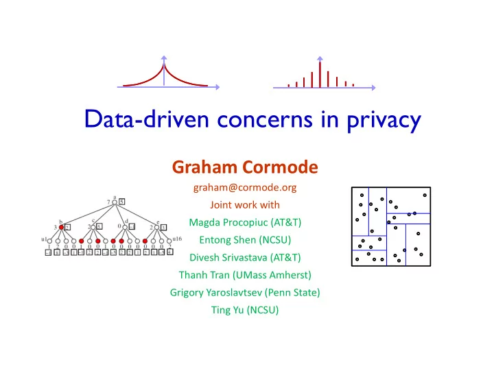
Data-driven concerns in privacy Graham Cormode graham@cormode.org - PowerPoint PPT Presentation
Data-driven concerns in privacy Graham Cormode graham@cormode.org graham@cormode.org Joint work with Magda Procopiuc (AT&T) Entong Shen (NCSU) Divesh Srivastava (AT&T) Thanh Tran (UMass Amherst) Grigory Yaroslavtsev (Penn State)
Data-driven concerns in privacy Graham Cormode graham@cormode.org graham@cormode.org Joint work with Magda Procopiuc (AT&T) Entong Shen (NCSU) Divesh Srivastava (AT&T) Thanh Tran (UMass Amherst) Grigory Yaroslavtsev (Penn State) Ting Yu (NCSU)
Outline ♦ Anonymization and Privacy models ♦ Non-uniformity of data ♦ Optimizing linear queries ♦ Predictability in data 2
The anonymization scenario 3
Data-driven privacy ♦ Much interest in private data release – Practical: release of AOL, Netflix data etc. – Research: hundreds of papers ♦ In practice, many data-driven concerns arise: – Efficiency / practicality of algorithms as data scales – Efficiency / practicality of algorithms as data scales – How to interpret privacy guarantees – Handling of common data features, e.g. sparsity – Ability to optimize for known query workload – Usability of output for general processing ♦ This talk: outline some efforts to address these issues 4
Differential Privacy [Dwork 06] ♦ Principle: released info reveals little about any individual – Even if adversary knows (almost) everything about everyone else! ♦ Thus, individuals should be secure about contributing their data – What is learnt about them is about the same either way ♦ Much work on providing differential privacy – Simple recipe for some data types e.g. numeric answers – Simple rules allow us to reason about composition of results – More complex for arbitrary data (exponential mechanism) ♦ Adopted and used by several organizations: – US Census, Common Data Project, Facebook (?)
Differential Privacy The output distribution of a differentially private algorithm changes very little whether or not any individual’s data is included in the input – so you should contribute your data A randomized algorithm K satisfies ε-differential privacy if: Given any pair of neighboring data sets, D 1 and D 2 , and S in Range(K): Pr[K(D 1 ) = S] ≤ e ε Pr[K(D 2 ) = S]
Achieving ε -Differential Privacy (Global) Sensitivity of publishing: s = max x,x’ |F(x) – F(x’)|, x, x’ differ by 1 individual E.g., count individuals satisfying property P: one individual changing info affects answer by at most 1; hence s = 1 For every value that is output: � Add Laplacian noise, Lap(ε/s): Or Geometric noise for discrete case: � Simple rules for composition of differentially private outputs: Given output O 1 that is ε 1 private and O 2 that is ε 2 private � (Sequential composition) If inputs overlap, result is ε 1 + ε 2 private � (Parallel composition) If inputs disjoint, result is max( ε 1 , ε 2 ) private
Outline ♦ Anonymization and Privacy models ♦ Non-uniformity of data ♦ Optimizing linear queries ♦ Predictability in data 8
Sparse Spatial Data [ICDE 2012] ♦ Consider location data of many individuals – Some dense areas (towns and cities), some sparse (rural) ♦ Applying DP naively simply generates noise – lay down a fine grid, signal overwhelmed by noise ♦ Instead: compact regions with sufficient number of points 9
Private Spatial decompositions quadtree kd-tree ♦ Build: adapt existing methods to have differential privacy ♦ Release: a private description of data distribution (in the form of bounding boxes and noisy counts) 10
Building a Private kd-tree ♦ Process to build a private kd-tree � Input: maximum height h , minimum leaf size L, data set � Choose dimension to split � Get (private) median in this dimension � Create child nodes and add noise to the counts � Recurse until: � Max height is reached � Noisy count of this node less than L � Budget along the root-leaf path has used up ♦ The entire PSD satisfies DP by the composition property 11
Building PSDs – privacy budget allocation ♦ Data owner specifies a total budget reflecting the level of anonymization desired ♦ Budget is split between medians and counts – Tradeoff accuracy of division with accuracy of counts ♦ Budget is split across levels of the tree ♦ Budget is split across levels of the tree – Privacy budget used along any root-leaf path should total ε Sequential composition Parallel composition 12
Privacy budget allocation ♦ How to set an ε i for each level? – Compute the number of nodes touched by a ‘typical’ query – Minimize variance of such queries – Optimization: min ∑ i 2 h-i / ε i 2 s.t. ∑ i ε i = ε – Solved by ε ∝ ( 2 (h-i) ) 1/3 ε : more to leaves – Solved by ε i ∝ ( 2 ε : more to leaves ) – Total error (variance) goes as 2 h / ε 2 ♦ Tradeoff between noise error and spatial uncertainty – Reducing h drops the noise error – But lower h increases the size of leaves, more uncertainty 13
Post-processing of noisy counts ♦ Can do additional post-processing of the noisy counts – To improve query accuracy and achieve consistency ♦ Intuition: we have count estimate for a node and for its children – Combine these independent estimates to get better accuracy – Make consistent with some true set of leaf counts – Make consistent with some true set of leaf counts ♦ Formulate as a linear system in n unknowns – Avoid explicitly solving the system – Expresses optimal estimate for node v in terms of estimates of ancestors and noisy counts in subtree of v – Use the tree-structure to solve in three passes over the tree – Linear time to find optimal, consistent estimates
Experimental study ♦ 1.63 million coordinates from US TIGER/Line dataset – Road intersections of US States ♦ Queries of different shapes, e.g. square, skinny ♦ Measured median relative error of 600 queries for each shape 15
Experimental study ♦ Effectiveness of geometric budget and post-processing – Relative error reduced by up to an order of magnitude – Most effective when limited privacy budget 16
Outline ♦ Anonymization and Privacy models ♦ Non-uniformity of data ♦ Optimizing linear queries ♦ Predictability in data 17
Optimizing Linear Queries [ICDE 2013] ♦ Linear queries capture many common cases for data release – Data is represented as a vector x – Want to release answers to linear combinations of entries of x – E.g. contingency tables in statistics – Model queries as matrix Q, want to know y=Qx – Model queries as matrix Q, want to know y=Qx 3 5 1 1 1 1 0 0 0 0 7 0 0 0 0 1 1 1 1 0 1 1 0 0 0 0 0 0 x= Q= 1 0 0 1 1 0 0 0 0 4 0 0 0 0 1 1 0 0 9 0 0 0 0 0 0 1 1 2 18
Answering Linear Queries ♦ Basic approach: – Answer each query in Q directly, and add uniform noise ♦ Basic approach is suboptimal – Especially when some queries overlap and others are disjoint ♦ Several opportunities for optimization: – Can assign different scales of noise to different queries – Can combine results to improve accuracy – Can ask different queries, and recombine to answer Q ( ) 1 1 1 1 0 0 0 0 0 0 0 0 1 1 1 1 1 1 0 0 0 0 0 0 Q= 0 0 1 1 0 0 0 0 0 0 0 0 1 1 0 0 0 0 0 0 0 0 1 1 19
The Strategy/Recovery Approach ♦ Pick a strategy matrix S – Compute z = Sx + v noise vector strategy on data – Find R so that Q = RS – Return y = Rz = Qx + Rv as the set of answers – Return y = Rz = Qx + Rv as the set of answers – Measure accuracy based on var(y) = var(Rv) ♦ Common strategies used in prior work: I: Identity Matrix C: Selected Marginals Q: Query Matrix H: Haar Wavelets F: Fourier Matrix P: Random projections 20
Step 1: Error Minimization ♦ Given Q, R, S, ε want to find a set of values { ε i } – Noise vector v has noise in entry i with variance 1/ ε i 2 ♦ Yields an optimization problem of the form: – Minimize ∑ i b i / ε i 2 (minimize variance) – Subject to ∑ |S | ε ≤ ε – Subject to ∑ i |S i,j | ε i ≤ ε (guarantee ε differential privacy) (guarantee ε differential privacy) ♦ The optimization is convex, can solve via interior point methods – Costly when S is large – We seek an efficient closed form for common strategies 21
Grouping Approach ♦ We observe that many strategies S can be broken into groups that behave in a symmetrical way – Rows in a group are disjoint (have zero inner product) – Non-zero values in group i have same magnitude C i ♦ All common strategies meet this grouping condition ♦ All common strategies meet this grouping condition – Identity (I), Fourier (F), Marginals (C), Projections (P), Wavelets (H) ♦ Simplifies the optimization: – A single constraint over the ε i ’s – New constraint: ∑ Groups i C i ε i = ε – Closed form solution via Lagrangian 22
Step 2: Optimal Recovery Matrix ♦ Given Q, S, { ε i }, find R so that Q=RS – Minimize the variance Var(Rz) = Var(RSx + Rv) = Var(Rv) ♦ Find an optimal solution by adapting Least Squares method ♦ This finds x’ as an estimate of x given z = Sx + v – Define Σ = Cov(z) = diag(2/ ε i Σ ε 2 2 ) and U = Σ -1/2 S Σ -1/2 – – OLS solution is x’ = (U T U ) -1 U T Σ -1/2 z ♦ Then R = Q(S T Σ -1 S) -1 S T Σ -1 ♦ Result: y = Rz = Qx’ is consistent—corresponds to queries on x’ – R minimizes the variance – Special case: S is orthonormal basis (S T = S -1 ) then R=QS T 23
Recommend
More recommend
Explore More Topics
Stay informed with curated content and fresh updates.
