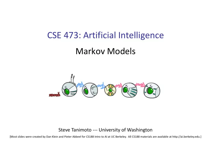

CSE 473: Artificial Intelligence Markov Models Steve Tanimoto --- University of Washington [Most slides were created by Dan Klein and Pieter Abbeel for CS188 Intro to AI at UC Berkeley. All CS188 materials are available at http://ai.berkeley.edu.]
Reasoning over Time or Space Often, we want to reason about a sequence of observations Speech recognition Robot localization User attention Medical monitoring Need to introduce time (or space) into our models
Markov Models Value of X at a given time is called the state X 1 X 2 X 3 X 4 Parameters: called transition probabilities or dynamics, specify how the state evolves over time (also, initial state probabilities) Stationarity assumption: transition probabilities the same at all times Same as MDP transition model, but no choice of action
Joint Distribution of a Markov Model X 1 X 2 X 3 X 4 Joint distribution: More generally: Questions to be resolved: Does this indeed define a joint distribution? Can every joint distribution be factored this way, or are we making some assumptions about the joint distribution by using this factorization?
Chain Rule and Markov Models X 1 X 2 X 3 X 4 From the chain rule, every joint distribution over can be written as: Assuming that and simplifies to the expression posited on the previous slide:
Chain Rule and Markov Models X 1 X 2 X 3 X 4 From the chain rule, every joint distribution over can be written as: Assuming that for all t : simplifies to the expression posited on the earlier slide:
Implied Conditional Independencies X 1 X 2 X 3 X 4 We assumed: and Do we also have ? Yes! Proof:
Markov Models Recap Explicit assumption for all t : Consequence, joint distribution can be written as: Implied conditional independencies: Past independent of future given the present i.e., if then: Additional explicit assumption: is the same for all t
Example Markov Chain: Weather States: X = {rain, sun} Initial distribution: 1.0 sun CPT P(X t | X t-1 ): Two new ways of representing the same CPT X t-1 X t P(X t |X t-1 ) 0.9 0.3 0.9 sun sun 0.9 sun sun rain sun 0.3 sun rain 0.1 0.1 rain sun 0.3 rain rain 0.7 rain rain 0.7 0.7 0.1
Example Markov Chain: Weather Initial distribution: 1.0 sun 0.9 0.3 rain sun 0.7 0.1 What is the probability distribution after one step?
Mini-Forward Algorithm Question: What’s P(X) on some day t? X 1 X 2 X 3 X 4 Forward simulation
Example Run of Mini-Forward Algorithm From initial observation of sun P( X 1 ) P( X 2 ) P( X 3 ) P( X 4 ) P( X ∞ ) From initial observation of rain P( X 4 ) P( X 1 ) P( X 2 ) P( X 3 ) P( X ∞ ) From yet another initial distribution P(X 1 ): … P( X 1 ) P( X ∞ ) [Demo: L13D1,2,3]
Video of Demo Ghostbusters Basic Dynamics
Video of Demo Ghostbusters Circular Dynamics
Video of Demo Ghostbusters Whirlpool Dynamics
Stationary Distributions For most chains: Stationary distribution: Influence of the initial distribution The distribution we end up with is called gets less and less over time. the stationary distribution of the chain The distribution we end up in is It satisfies independent of the initial distribution
Example: Stationary Distributions Question: What’s P(X) at time t = infinity? X 1 X 2 X 3 X 4 X t-1 X t P(X t |X t-1 ) sun sun 0.9 sun rain 0.1 rain sun 0.3 rain rain 0.7 Also:
Application of Stationary Distribution: Web Link Analysis PageRank over a web graph Each web page is a state Initial distribution: uniform over pages Transitions: With prob. c, uniform jump to a random page (dotted lines, not all shown) With prob. 1-c, follow a random outlink (solid lines) Stationary distribution Will spend more time on highly reachable pages E.g. many ways to get to the Acrobat Reader download page Somewhat robust to link spam Google 1.0 returned the set of pages containing all your keywords in decreasing rank, now all search engines use link analysis along with many other factors (rank actually getting less important over time)
Recommend
More recommend