CSE 421 Course Overview / Complexity 1 Administrativia Stuffs HW1 - PowerPoint PPT Presentation
CSE 421 Course Overview / Complexity 1 Administrativia Stuffs HW1 is out! It is due Thursday April 11 at 5:00 Please submit to Canvas Late Submission: Coordinate with me How to submit? Submit a separate file for each problem
CSE 421 Course Overview / Complexity 1
Administrativia Stuffs HW1 is out! It is due Thursday April 11 at 5:00 Please submit to Canvas Late Submission: Coordinate with me How to submit? • Submit a separate file for each problem • Double check your submission before the deadline!! • For hand written solutions, take a picture, turn it into pdf and submit Guidelines: • Always justify your answer • You can collaborate, but you must write solutions on your own • Your proofs should be clear, well-organized, and concise. Spell out main idea. • Sanity Check: Make sure you use assumptions of the problem 2
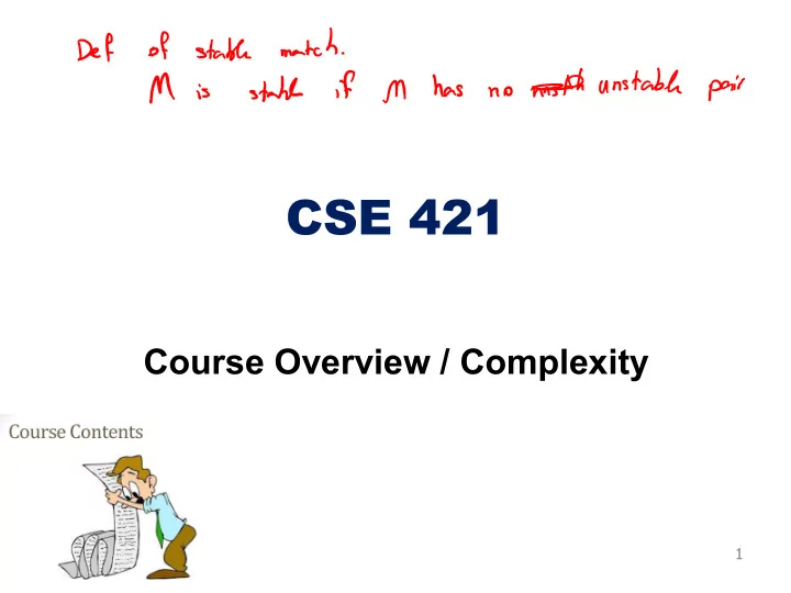
Extensions: Matching Residents to Hospitals Men » hospitals, Women » med school residents. • Variant 1: Some participants declare others as unacceptable. • Variant 2: Unequal number of men and women. e.g. A resident not interested in Cleveland • Variant 3: Limited polygamy. e.g. A hospital wants to hire 3 residents Def: Matching S is unstable if there is hospital h and resident r s.t. • h and r are acceptable to each other; and • either r is unmatched, or r prefers h to her assigned hospital; and • either h does not have all its places filled, or h prefers r to at least one of its assigned residents. 3
Lessons Learned • Powerful ideas learned in course. • Isolate underlying structure of problem. • Create useful and efficient algorithms. • Potentially deep social ramifications. [legal disclaimer] • Historically, men propose to women. Why not vice versa? • Men: propose early and often. • Men: be more honest. • Women: ask out the guys. • Theory can be socially enriching and fun! 4
“The Match”: Doctors and Medical Residences • Each medical school graduate submits a ranked list of hospital where he wants to do a residency • Each hospital submits a ranked list of newly minted doctors • A computer runs stable matching algorithm (extended to handle polygamy) • Until recently, it was hospital-optimal. 5
History 1900 • Idea of hospital having residents (then called “interns”) 1900-1940s • Intense competition among hospitals • Each hospital makes offers independently • Process degenerates into a race; hospitals advancing date at which they finalize binding contracts 1944 • Medical schools stop releasing info about students before a fixed date 1945-1949 • Hospitals started putting time limits on offers • Time limits down to 12 hours; lots of unhappy people 6
“The Match” 1950 • NICI run a centralized algorithm for a trial run • The pairing was not stable, Oops!! 1952 • The algorithm was modified and adopted. It was called the Match. • The first matching produced in April 1952 7
Five Representative Problems 1. Interval Scheduling 2. Weighted Interval Scheduling 3. Bipartite Matching 4. Independent Set Problem 5. Competitive Facility Location 8
Interval Scheduling Input: Given a set of jobs with start/finish times Goal: Find the maximum cardinality subset of jobs that can be run on a single machine. a b b c d e e f g h h Time 0 1 2 3 4 5 6 7 8 9 10 11 9
Interval Scheduling Input: Given a set of jobs with start/finish times Goal: Find the maximum weight subset of jobs that can be run on a single machine. 23 12 20 26 13 20 11 16 Time 0 1 2 3 4 5 6 7 8 9 10 11 10
Bipartite Matching Input: Given a bipartite graph Goal: Find the maximum cardinality matching A 1 B 2 C 3 D 4 E 5 11
Independent Set Input: A graph Goal: Find the maximum independent set Subset of nodes that no two joined by an edge 2 1 4 5 3 7 6 12
Competitive Facility Location Input: Graph with weight on each node Game: Two competing players alternate in selecting nodes. Not allowed to select a node if any of its neighbors have been selected . Goal. Does player 2 have a strategy which guarantees a total value of ! no matter what player 1 does ? 10 1 5 15 5 1 5 1 15 10 Second player can guarantee 20, but not 25. 13
Five Representative Problems Variation of a theme: Independent set Problem 1. Interval Scheduling ! log ! greedy algorithm 2. Weighted Interval Scheduling ! log ! dynamic programming algorithm 3. Bipartite Matching ! % maximum flow based algorithm 4. Independent Set Problem: NP-complete 5. Competitive Facility Location: PSPACE-complete 14
Defining Efficient Algorithms 15
Defining Efficiency “Runs fast on typical real problem instances” Pros: • Sensible, • Bottom-line oriented Cons: • Moving target (diff computers, programming languages) • Highly subjective (how fast is “fast”? What is “typical”?) 16
Measuring Efficiency Time » # of instructions executed in a simple programming language only simple operations (+,*,-,=,if,call,…) each operation takes one time step each memory access takes one time step no fancy stuff (add these two matrices, copy this long string,…) built in; write it/charge for it as above 17
Time Complexity Problem: An algorithm can have different running time on different inputs Solution: The complexity of an algorithm associates a number T(N) , the “time” the algorithm takes on problem size N . On which inputs of size N ? Mathematically, T is a function that maps positive integers giving problem size to positive integers giving number of steps 18
Time Complexity (N) Worst Case Complexity: max # steps algorithm takes on any input of size N This Couse Average Case Complexity: avg # steps algorithm takes on inputs of size N Best Case Complexity: min # steps algorithm takes on any input of size N 19
Why Worst-case Inputs? • Analysis is typically easier • Useful in real-time applications e.g., space shuttle, nuclear reactors) • Worst-case instances kick in when an algorithm is run as a module many times e.g., geometry or linear algebra library • Useful when running competitions e.g., airline prices • Unlike average-case no debate about the right definition 20
Time Complexity on Worst Case Inputs T ( N ) 2! log 2 ! Time ! log % ! Problem size N 21
O-Notation Given two positive functions f and g • f(N) is O(g(N)) iff there is a constant c > 0 s.t., f(N) is eventually always £ c g(N) • f(N) is W (g(N)) iff there is a constant e > 0 s.t., f(N) is ³ e g(N) for infinitely • f(N) is Q (g(N)) iff there are constants c 1 , c 2 >0 so that eventually always c 1 g(N) £ f(N) £ c 2 g(N) 22
Asymptotic Bounds for common fns • Polynomials: ! " + ! $ % + ⋯ + ! ' % ' is ( % ' • Logarithms: log , % = ((log / %) for all constants !, 2 > 0 • Logarithms: log grows slower than every polynomial For all 5 > 0 , log % = ((% 6 ) • % log % = ( % $."$ 23
Efficient = Polynomial Time An algorithm runs in polynomial time if T(n)=O(n d ) for some constant d independent of the input size n. Why Polynomial time? If problem size grows by at most a constant factor then so does the running time • E.g. T ( 2N ) £ c ( 2N ) k £ 2 k ( cN k ) • Polynomial-time is exactly the set of running times that have this property Typical running times are small degree polynomials, mostly less than N 3 , at worst N 6 , not N 100 24
Why it matters? #atoms in universe < 2 "#$ • Life of the universe < 2 %# seconds • A CPU does < 2 &$ operations a second • If every atom is a CPU, a 2 ' time ALG cannot solve n=350 if we start at Big-Bang. not only get very big, but do so abruptly , which likely yields erratic performance on small instances 25
Why “Polynomial”? Point is not that n 2000 is a practical bound, or that the differences among n and 2n and n 2 are negligible. Rather, simple theoretical tools may not easily capture such differences, whereas exponentials are qualitatively different from polynomials, so more amenable to theoretical analysis. • “My problem is in P” is a starting point for a more detailed analysis • “My problem is not in P” may suggest that you need to shift to a more tractable variant 26
Recommend
More recommend
Explore More Topics
Stay informed with curated content and fresh updates.
