CS681: Advanced Topics in Computational Biology Week 2, Lecture 1 - PowerPoint PPT Presentation
CS681: Advanced Topics in Computational Biology Week 2, Lecture 1 Can Alkan EA224 calkan@cs.bilkent.edu.tr http://www.cs.bilkent.edu.tr/~calkan/teaching/cs681/ Microarrays Targeted approach for: SNP / indel detection/genotyping
CS681: Advanced Topics in Computational Biology Week 2, Lecture 1 Can Alkan EA224 calkan@cs.bilkent.edu.tr http://www.cs.bilkent.edu.tr/~calkan/teaching/cs681/
Microarrays Targeted approach for: SNP / indel detection/genotyping Screen for mutations that cause disease Gene expression profiling Which genes are expressed in which tissue? Which genes are expressed “together” Gene regulation (chromatin immunoprecipitation) Fusion gene profiling Alternative splicing CNV discovery & genotyping …. 50K to 4.3M probes per chip
Microarray experiments Produce DNA library If working on RNA, then make cDNA from mRNA Attach phosphor (marker) to DNA/cDNA Different color phosphors are available to compare many samples at once Hybridize DNA/cDNA over the micro array Scan the microarray with a phosphor- illuminating laser Illumination reveals hybridization Scan microarray multiple times for the different color phosphor’s
DNA Microarray Tagged probes become hybridized Millions of DNA strands build up on each location. to the DNA chip’s microarray. http://www.affymetrix.com/corporate/media/image_library/image_library_1.affx
Image processing and normalization: what is microarray data? Microarray data is summary information from image files that come out of the scanner. Image processing: line up grids, flag bad spots, quantify. Segmentation & clustering algorithms
Data Slides: 11120c01 -11121c01 3-AT vs. 2 2 P-value < 0.01 log 10 (ratio) 1.5 No drug 1 1 0.5 0 0 -0.5 -1 -1 -1.5 -2 -2 -2 -1 0 1 2 wild-type vs. 2 2 P-value < 0.01 1.5 wild-type log 10 (ratio) 1 1 0.5 0 0 -0.5 -1 -1 -1.5 -2 -2 -2 -1 0 1 2 log 10 (average intensity)
Microarray Vendors Illumina Omni5 chip – 1000 Genomes: 4.3M markers Agilent NimbleGen Affymetrix All similar principles; different markers Custom designs can be made
Using Microarrays (SNP genotyping) Microarrays designed with oligonucleotides that harbor “target” SNPs. Comprehensively and rapidly study single nucleotide polymorphisms in human genomes Current SNP arrays feature 2 million genetic markers Analysis based on image processing and statistical methods
Microarray Experiments (gene expression) www.affymetrix.com
Using Microarrays (gene expression) • Track the sample over a period of time to see gene expression over time • Track two different samples under the same conditions to see the difference in gene expressions Each box represents one gene’s expression over time
Using Microarrays (cont’d) Green : expressed only from control Red : expressed only from experimental cell Yellow : equally expressed in both samples Black : NOT expressed in either control or experimental cells
Clustering algorithms Clustering can be used for: Primary analysis: cluster signals in microarray image to Merge real signals from the same molecule Separate real signals from noise Secondary analysis: Grouping probes: which probes are hybridized together? Good for probes that might be repetitive in the genome/transcriptome Gene expression: which genes are expressed together? Many other bioinformatic applications exist
Homogeneity and Separation Principles Homogeneity: Elements within a cluster are close to each other Separation: Elements in different clusters are further apart from each other …clustering is not an easy task! Given these points a clustering algorithm might make two distinct clusters as follows
Bad Clustering This clustering violates both Homogeneity and Separation principles Close distances from points in separate clusters Far distances from points in the same cluster
Good Clustering This clustering satisfies both Homogeneity and Separation principles
Clustering Algorithms • Hierarchical c a b h e d f a b d e f c g h g c • K-means c2 a b h e d c3 c1 f d e f a b c g h g slide credits: M. Kellis
Hierarchical clustering Bottom-up algorithm: Initialization: each point in a separate cluster c At each step: a b Choose the pair of closest clusters Merge h e d The exact behavior of the algorithm f g depends on how we define the distance CD(X,Y) between clusters X and Y Avoids the problem of specifying the number of clusters slide credits: M. Kellis
Distance between clusters h e CD(X,Y)=min x X, y Y D(x,y) d f Single-link method g CD(X,Y)=max x X, y Y D(x,y) h e d Complete-link method f g CD(X,Y)=avg x X, y Y D(x,y) Average-link method h e d CD(X,Y)=D( avg(X) , avg(Y) ) f g Centroid method h e d f g slide credits: M. Kellis
Hierarchical Clustering
Hierarchical Clustering: Example
Hierarchical Clustering: Example
Hierarchical Clustering: Example
Hierarchical Clustering: Example
Hierarchical Clustering: Example
Hierarchical Clustering Algorithm Hierarchical Clustering ( d , n ) 1. Form n clusters each with one element 2. Construct a graph T by assigning one vertex to each cluster 3. while there is more than one cluster 4. 4. Find the two closest clusters C 1 and C 2 5. Merge C 1 and C 2 into new cluster C with |C 1 | + |C 2 | elements 6. Compute distance ce from C to a all o other r cluster ters 7. 7. Add a new vertex C to T and connect to vertices C 1 and C 2 8. Remove rows and columns of d corresponding to C 1 and C 2 9. Add a row and column to d corrsponding to the new cluster C 10. return T 11. The algorithm takes a n x n distance matrix d of pairwise distances between points as an input.
Hierarchical Clustering Algorithm Hierarchical Clustering ( d , n ) 1. Form n clusters each with one element 2. Construct a graph T by assigning one vertex to each cluster 3. while there is more than one cluster 4. 4. Find the two closest clusters C 1 and C 2 5. Merge C 1 and C 2 into new cluster C with |C 1 | + |C 2 | elements 6. Compute distance ce from C to a all o other r cluster ters 7. 7. Add a new vertex C to T and connect to vertices C 1 and C 2 8. Remove rows and columns of d corresponding to C 1 and C 2 9. Add a row and column to d corrsponding to the new cluster C 10. return T 11. Different ways to define distances between clusters may lead to different clusterings
K-Means Clustering Algorithm Each cluster X i has a center c i Define the clustering cost criterion COST(X 1 ,…X k ) = ∑ Xi ∑ x Xi |x – c i | 2 c Algorithm tries to find clusters X 1 …X k and c2 a b centers c 1 …c k that minimize COST K-means algorithm: c3 h e Initialize centers d c1 f Repeat: g Compute best clusters for given centers → Attach each point to the closest center Compute best centers for given clusters → Choose the centroid of points in cluster Until the changes in COST are “ small ” slide credits: M. Kellis
K-Means Algorithm Randomly Initialize Clusters
K-Means Algorithm Assign data points to nearest clusters
K-Means Algorithm Recalculate Clusters
K-Means Algorithm Recalculate Clusters
K-Means Algorithm Repeat
K-Means Algorithm Repeat
K-Means Algorithm Repeat … until convergence Time: O(KNM) per iteration N: #genes M: #conditions
K-Means Greedy Algorithm ProgressiveGreedyK-Means(k) 1. Select an arbitrary partition P into k clusters 2. while hile forever 3. 3. bestChange 0 4. for every cluster C 5. 5. for every element i not in C 6. 6. if if moving i to cluster C reduces its clustering cost 7. 7. if if (cost(P) – cost(P i C ) > bestChange 8. bestChange cost(P) – cost(P i C ) 9. i * I 10. C * C 11. if if bestChange > 0 12. 12. Change partition P by moving i * to C * 13. else 14. return urn P 15. 15.
Clustering: Gene ontology (GO) Catalogue for genes, gene products, gene annotations across all species Clustered genes with respect to biological processes they were involved in Single gene can appear in multiple processes
GO-Biological Process categories # annotated genes (mouse) metabolism 1548 Very Broad development 2341 vision 163 Broad CNS development 137 eye morphogenesis 21 ATP biosynthesis 36 Mid-level pigment metabolism 25 striated muscle contraction 33 eye pigment metabolism 3 Narrow 4 insulin secretion
Recommend
More recommend
Explore More Topics
Stay informed with curated content and fresh updates.
