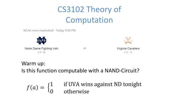
CS3102 Theory of Computation Warm up: Is this function computable - PowerPoint PPT Presentation

CS3102 Theory of Computation Warm up: Is this function computable with a NAND-Circuit? 𝑔 𝑏 = 1 if UVA wins against ND tonight 0 otherwise

Logistics • Quiz 3 out – Due Thursday • Exercise 3 is out – Last exercise before midterm 2

Last Time • Showing that NAND/AON can compute any finite function • Started showing how we could have a function that simulates programs 3

How are programs run? • Have a table of variables • Execute code in sequence • Update values in table • Return a value from the table 4

Programs as Bits • To evaluate a program with another program, we need to convert the first program into bits 1. Number each variable (first n go to input, last m to outputs) 2. Represent each line as 3 numbers (outvar, in1, in2) 3. Represent program as (n,m,[Lines]) Variable Number a 0 (2,0,0) b 1 (3,1,1) temp1 2 (4,2,3) temp2 3 (2,1,[(2,0,0),(3,1,1),(4,2,3)]) return 4 5

XOR to bits Variable Number 𝑜 = 𝑛 = 𝑡 = Total bits = 6

XOR to bits Variable Number a 0 b 1 u 2 𝑜 = 2 v 3 𝑛 = 1 w 4 𝑡 = 4 return 5 Total bits = 3 [numbers per line] ⋅ 3 [bits per number] ⋅ 4[lines] + 6 [length of 𝑜 + 𝑛 ] 7

How big is this? 1. Number each variable ⌈log 2 3𝑡⌉ bits each 2. Represent each line as 3 numbers (outvar, in1, in2) 3𝑡 ⋅ ⌈log 2 3𝑡⌉ bits 3. Represent program as (n,m,[Lines]) 2⌈log 2 𝑡⌉ bits 𝑇 𝑡 ≤ 4𝑡⌈log 2 3𝑡⌉ ℓ = ⌈log 2 3𝑡⌉ 8

Defining EVAL 𝐹𝑊𝐵𝑀 𝑡,𝑜,𝑛 : 0,1 𝑇 𝑡 +𝑜 → 0,1 𝑛 Input: bit string representing a program (first 𝑇(𝑡) bits) plus input values (remaining 𝑜 bits) Output: the result of running the represented program on the provided input, or 𝑛 0's if there's a "compile error" 9

𝑜 = 2 Defining the EVAL function 𝑛 = 1 Variable Value Representation: 0 (2, 0, 1), (3, 0, 2), (4, 1, 2), 1 (5, 3, 4) 2 Input: 0, 1 3 4 5 10

Psuedocode for EVAL 𝑈 • Table 𝑈 : – holds variables and their values • 𝐻𝐹𝑈(𝑈, 𝑗) – Returns the bit of 𝑈 associated with variable 𝑗 • 𝑉𝑄𝐸𝐵𝑈𝐹(𝑈, 𝑗, 𝑐) – Returns a new table such that variable 𝑗 's value has been changed to 𝑐 11

Psuedocode for EVAL • Input: Let 𝑈 be table of size 𝑢 Numbers 𝑜 , 𝑛 , 𝑡 , 𝑢 For 𝑗 in range( 𝑜 ): – representing the number of 𝑈 = UPDATE( 𝑈 , 𝑗 , 𝑦[𝑗] ) inputs, outputs, variables, For ( 𝑗 , 𝑘 , 𝑙 ) in 𝑀 : and lines respectively 𝑏 = GET( 𝑈 , 𝑘 ) 𝑀 , a list of triples – 𝑐 = GET( 𝑈 , 𝑙 ) representing the program 𝑈 = UPDATE( 𝑈 , 𝑗 , NAND( 𝑏 , 𝑐 )) A string 𝑦 to be given as input – For 𝑗 in range( 𝑛 ): to the program 𝑍 [ 𝑗 ] = GET( 𝑈 , 𝑢 − 𝑛 + 𝑗 ) • Output: Return 𝑍 – Evaluation of the program represented by 𝑀 when run on input 𝑦 12

EVAL in NAND • Next we implement 𝐹𝑊𝐵𝑀 𝑡,𝑜,𝑛 using NAND 13

𝐻𝐹𝑈(𝑈, 𝑗) • Get the bit at “row” 𝑗 of 𝑈 • Look familiar? • How many gates to implement? 14

UPDATE 𝑉𝑄𝐸𝐵𝑈𝐹 ℓ : 0,1 𝑡 ℓ +ℓ+1 → 0,1 2 ℓ • To change index 𝑗 of table 𝑈 to bit 𝑐 • For every index except 𝑗 , return the same value • For index 𝑗 , return b instead • Define 𝐹𝑅𝑉𝐵𝑀 𝑘 : 0,1 ℓ → {0,1} which returns 1 if the input binary number is equal to j Note: 𝐹𝑅𝑉𝐵𝑀 𝑘 can be done in 𝑑 ⋅ ℓ gates 15

UPDATE pseudocode For 𝑘 in range( 2 ℓ ): 𝑏 = 𝐹𝑅𝑉𝐵𝑀𝑇 𝑘 (𝑗) Runs 2 ℓ times 𝑜𝑓𝑥𝑈[𝑘 ] = 𝐽𝐺(𝑏, 𝑐, 𝑈[𝑘]) Return 𝑜𝑓𝑥𝑈 16

Conclusion • What we know: – We can compute any finite function with circuits – We can compute a function to evaluate programs of a certain size • Big question: – How expensive are functions? – Some are more expensive than others, how big could they get? – If I wanted to be able to evaluate a program for any function 0,1 𝑜 → {0,1} , how big would the eval circuit need to be? 17

Complexity • The "complexity" of a function: – Measure of the resources required to compute that function • Complexity Class: – A set of functions defined by a complexity measure 18

Categorizing Functions by Circuit Size • No functions require more than 𝑑𝑛2 𝑜 gates – Proved last class • Some functions require much less – E.g. IF • Observation: some functions are more "complicated" than others! • Idea: categorize functions by resources required to implement them using a particular computing model 19

SIZE • 𝑇𝐽𝑎𝐹(𝑡) : The set of all functions that can be implemented by a circuit of at most s NAND gates 𝑇𝐽𝑎𝐹(1000𝑛2 𝑜 ) Contains all functions 𝑔: 0,1 𝑜 → 0,1 𝑛 • TCS also uses: – 𝑇𝐽𝑎𝐹 𝑜,𝑛 𝑡 :The set of all 𝑜 -input, 𝑛 -output functions that can be implemented with at most 𝑡 NAND gates – 𝑇𝐽𝑎𝐹 𝑜 𝑡 : The set of all 𝑜 -input, 1 -output functions that can be implemented with at most 𝑡 NAND gates 20

Comparing Classes If 𝑦 ≤ 𝑧 , then 𝑇𝐽𝑎𝐹 𝑡 ⊆ 𝑇𝐽𝑎𝐹(𝑧) 21

Theorem • Let 𝑇𝐽𝑎𝐹 𝐵𝑃𝑂 𝑡 represent the set of all functions that can be computed using at most 𝑡 AND/OR/NOT gates 𝑇𝐽𝑎𝐹 𝑡 2 ⊆ 𝑇𝐽𝑎𝐹 𝐵𝑃𝑂 𝑡 ⊆ 𝑇𝐽𝑎𝐹 3𝑡 22

Proof 𝑇𝐽𝑎𝐹 𝑡 2 ⊆ 𝑇𝐽𝑎𝐹 𝐵𝑃𝑂 𝑡 ⊆ 𝑇𝐽𝑎𝐹 3𝑡 23

O, Ω, Θ • Groups functions together • Each uses a function as a bound for other functions • O (Big-Oh): – O(f(n)) = the set of all functions "asymptotically upper-bounded" by f • Ω (Big -Omega): – Ω(f(n)) = the set of all functions "asymptotically lower-bounded" by f • Θ (Big -Theta): – Θ(f(n)) = the set of all functions "asymptotically tight -bounded" by f 24

25

Definitions • 𝑃(𝑕 𝑜 ) • At most within constant of 𝑕 for large 𝑜 • {𝑔: ℝ → ℝ|∃ constants 𝑑, 𝑜 0 > 0 s.t. ∀𝑜 > 𝑜 0 , 𝑔 𝑜 ≤ 𝑑 ⋅ 𝑕(𝑜)} • Ω(𝑕 𝑜 ) • At least within constant of 𝑕 for large 𝑜 • {𝑔: ℝ → ℝ|∃ constants 𝑑, 𝑜 0 > 0 s.t. ∀𝑜 > 𝑜 0 , 𝑔 𝑜 ≥ 𝑑 ⋅ 𝑕(𝑜)} • Θ 𝑕 𝑜 • “ Tightly ” within constant of 𝑕 for large 𝑜 • Ω 𝑕 𝑜 ∩ 𝑃(𝑕 𝑜 ) 26

Showing Big-Oh • To show: 𝑜 log 𝑜 ∈ 𝑃 𝑜 2 27

Showing Big-Omega • To Show: 2 𝑜 ∈ Ω 𝑜 2 28

Showing Big-Theta • To Show: log 𝑦 𝑜 = Θ log 𝑧 𝑜 29