CS171 Visualization Alexander Lex alex@seas.harvard.edu Tables - PowerPoint PPT Presentation
CS171 Visualization Alexander Lex alex@seas.harvard.edu Tables Part II [xkcd] Next Week Reading: VAD, Chapters 9 Lecture 11: Text & Documents Lecture 12: Homework 3 Design Studio Sections: view coordination, linking & brushing
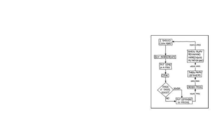
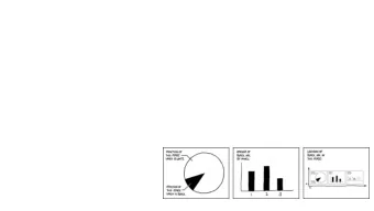
CS171 Visualization Alexander Lex alex@seas.harvard.edu Tables Part II [xkcd]
Next Week Reading: VAD, Chapters 9 Lecture 11: Text & Documents Lecture 12: Homework 3 Design Studio Sections: view coordination, linking & brushing Updates Design Studio moved to Thursday Project Proposal moved to HW 4
Tables & Multi- Dimensional Data
Comparisons
Direction Nicolas Rapp
Plot Change Instead https://eagereyes.org/basics/baselines
Trends Over Time http://xkcd.com/605/
Bars vs. Lines Lines imply connections & sampling from continuous data. Do not use for categorical data. Zacks 1999
Baseline Problem (again) True Baseline Clipped Baseline Plotting Change https://eagereyes.org/basics/baselines
Linear vs. Logarithmic Scale Linear Scale Log Scale http://xkcd.com/1162/ Apple Stock Price http://finance.yahoo.com/echarts?s=AAPL
Aspect Ratios Rule of Thumb: Banking to 45º (average line slope: 45º) eagereyes.org
Correlations
Scatterplots
Overplotting alpha = 1/100
Compositions
Stacked Bar Chart
Comparison of bar chart types Pie Chart Stacked bar chart Layered Bar Chart Small Multiples Grouped Bar Chart Streit & Gehlenborg, PoV, Nature Methods, 2014
Stacked Area Chart http://stackoverflow.com/questions/2225995/how-can-i-create-stacked-line-graph-with-matplotlib
100% Stacked Area Chart http://stackoverflow.com/questions/16875546/create-a-100-stacked-area-chart-with-matplotlib
Stacked Area vs. Line Graphs leancrew.com & Practically Efficient
Distributions
Histogram # passengers #bins hard to predict make interactive! age rule of thumb: #bins = sqrt(n) 10 Bins # passengers age 20 Bins
Box Plots aka Box-and-Whisker Plot Wikipedia
Comparison Streit & Gehlenborg, PoV, Nature Methods, 2014
Showing Expected Values & Uncertainty Error Bars Considered Harmful: Exploring Alternate Encodings for Mean and Error Michael Correll, and Michael Gleicher
Highdimensional Data
What is High-dimensional Data? Age Gender Height Tabular data, containing Bob 25 M 181 rows (items) Alice 22 F 185 Chris 19 M 175 columns (attributes or items) rows >> columns
High-Dimensional Data Visualization Homogeneity Same data type? How many dimensions? Same scales? ~50 – tractable with “just” vis ~1000 – need analytical methods Age Gender Height How many records? Bob 25 M 181 ~ 1000 – “just” vis is fine Alice 22 F 185 Chris 19 M 175 >> 10,000 – need analytical methods BPM 1 BPM 2 BPM 3 Bob 65 120 145 Alice 80 135 185 Chris 45 115 135
Analytic Component Multidimensional Scaling Scatterplot Matrices [Doerk 2011] [Bostock] Pixel-based visualizations / heat maps Parallel Coordinates [Bostock] [Chuang 2012] no / little analytics strong analytics component
Geometric Methods
Parallel Coordinates (PC) Inselberg 1985 Axes represent attributes Lines connecting axes represent items X A A B B B A Y X Y
Parallel Coordinates Each axis represents dimension Lines connecting axis represent records Suitable for all tabular data types heterogeneous data
PC Limitation: Scalability to Many Dimensions 500 axes
PC Limitation: Scalability to Many Items Solutions: Transparency Bundling, Clustering Sampling
PC Limitations Correlations only between adjacent axes Solution: Interaction Brushing Let user change order
PC Limitation: Ambiguity Solutions: Brushing Curves Graham and Kennedy 2003
Parallel Coordinates Algorithmic support: Shows primarily relationships between adjacent axis Choosing dimensions Limited scalability (~50 Choosing order dimensions, ~1-5k records) Clustering & aggregating Transparency of lines Interaction is crucial records Axis reordering Brushing Filtering http://bl.ocks.org/jasondavies/1341281
Star Plot [Coekin1969] Similar to parallel coordinates Radiate from a common origin http://www.itl.nist.gov/div898/handbook/eda/section3/starplot.htm http://bl.ocks.org/kevinschaul/raw/8833989/ http://start1.jpl.nasa.gov/caseStudies/autoTool.cfm
Multiple Line Charts http://square.github.io/cubism/
Combining Various Charts
Scatterplot Matrices (SPLOM) Matrix of size d*d Each row/column is one dimension Each cell plots a scatterplot of two dimensions
Scatterplot Matrices Limited scalability (~20 Algorithmic approaches: dimensions, ~500-1k Clustering & aggregating records) records Brushing is important Choosing dimensions Often combined with “Focus Choosing order Scatterplot” as F+C technique
SPLOM Aggregation - Heat Map Datavore: http://vis.stanford.edu/projects/datavore/splom/
SPLOM F+C, Navigation [Elmqvist]
Flexible Linked Axes (FLINA) Claessen & van Wijk 2011
Web-based implementation of FLINA concept http://vis.pku.edu.cn/mddv/val/ ¡
Connected Charts Viau ¡& ¡McGuffin ¡2012 ¡
Domino origin ARTISTS Australia Europe North America studio albums WcountH first album WyearH continent Barbados Rihanna Ireland U2 Sweden ABBA Elton John UK The Beatles number one hits Whitney Houston The Black Eyed Peas Britney Spears start of Eminem US career WyearH Michael Jackson Madonna inactive active Elvis Presley Netherlands career status Germany Australia Sweden Canada France Austria Ireland Span Italy US UK COUNTRIES in business at first album 5 Artists sold albums WabsoluteH gender male group female inactive gender ∩ inactive 5 Countries population WmillionH Artists 0 12 Countries 1 12 Gratzl ¡et ¡al. ¡2014 ¡
Data Reduction Sampling Filtering Don’t show every element, show a Define criteria to remove data, e.g., (random) subset minimum variability > / < / = specific value for one dimension Efficient for large dataset consistency in replicates, … Apply only for display purposes Can be interactive, combined with Outlier-preserving approaches sampling [Ellis & Dix, 2006]
Filter Example http://square.github.io/crossfilter/
Pixel Based Methods
Pixel Based Displays Each cell is a “pixel”, value encoded in color / value Meaning derived from ordering If no ordering inherent, clustering is used Scalable – 1 px per item Good for homogeneous data same scale & type [Gehlenborg & Wong 2012]
3D Pitfall: Occlusion & Perspective [Gehlenborg and Wong, Nature Methods, 2012]
3D Pitfall: Occlusion & Perspective [Gehlenborg and Wong, Nature Methods, 2012]
Heterogeneous Data? [Verhaak 2012]
Bad Color Mapping
Good Color Mapping
Color is relative!
Clustering Classification of items into “similar” Hierarchical Algorithms bins Produce “similarity tree” – Based on similarity measures dendrogram Euclidean distance, Pearson Bi-Clustering correlation, ... Clusters dimensions & records Partitional Algorithms divide data into set of bins Fuzzy clustering # bins either manually set (e.g., k- allows occurrence of elements means) or automatically determined in multiples clusters (e.g., affinity propagation)
Clustering Applications Clusters can be used to order (pixel based techniques) brush (geometric techniques) aggregate Aggregation cluster more homogeneous than whole dataset statistical measures, distributions, etc. more meaningful
Clustered Heat Map
F+C Approach, with Dendrograms [Lex, PacificVis 2010]
Cluster Comparison
Aggregation
Design Critique
EdgeMaps: http://goo.gl/q8Cv7t http://mariandoerk.de/edgemaps/demo/#music
Dimensionality Reduction
Dimensionality Reduction Reduce high dimensional to lower dimensional space Preserve as much of variation as possible Plot lower dimensional space Principal Component Analysis (PCA) linear mapping, by order of variance
PCA Example – CS 171 Project 2013 http://mu-8.com/ [Mercer & Pandian]
Multidimensional Scaling Nonlinear, better suited for some DS Popular for text analysis [Doerk 2011]
Can we Trust Dimensionality Reduction? Topical distances between departments in Topical distances between the selected a 2D projection Petroleum Engineering and the others. [Chuang et al., 2012] http://www-nlp.stanford.edu/projects/dissertations/browser.html
Recommend
More recommend
Explore More Topics
Stay informed with curated content and fresh updates.
![CS171 Visualization Alexander Lex alex@seas.harvard.edu Tables [xkcd] This Week Reading: VAD,](https://c.sambuz.com/986063/cs171-visualization-s.webp)
![CS171 Visualization Alexander Lex alex@seas.harvard.edu Graphs [xkcd] This Week Reading: VAD,](https://c.sambuz.com/709269/cs171-visualization-s.webp)
![CS171 Visualization Alexander Lex alex@seas.harvard.edu Graphs Part II [xkcd] This Week](https://c.sambuz.com/723696/cs171-visualization-s.webp)
![CS171 Visualization Alexander Lex alex@seas.harvard.edu [xkcd] vi su al i za tion](https://c.sambuz.com/744411/cs171-visualization-s.webp)
![CS171 Visualization Alexander Lex alex@seas.harvard.edu Maps [xkcd] Homework 2 Review Grade](https://c.sambuz.com/767293/cs171-visualization-s.webp)
![CS171 Visualization Alexander Lex alex@seas.harvard.edu Design Guidelines Tasks [xkcd] Next](https://c.sambuz.com/864402/cs171-visualization-s.webp)



![CS-5630 / CS-6630 Visualization Tables Alexander Lex alex@sci.utah.edu [xkcd] dataset types](https://c.sambuz.com/935555/cs-5630-cs-6630-visualization-tables-s.webp)
