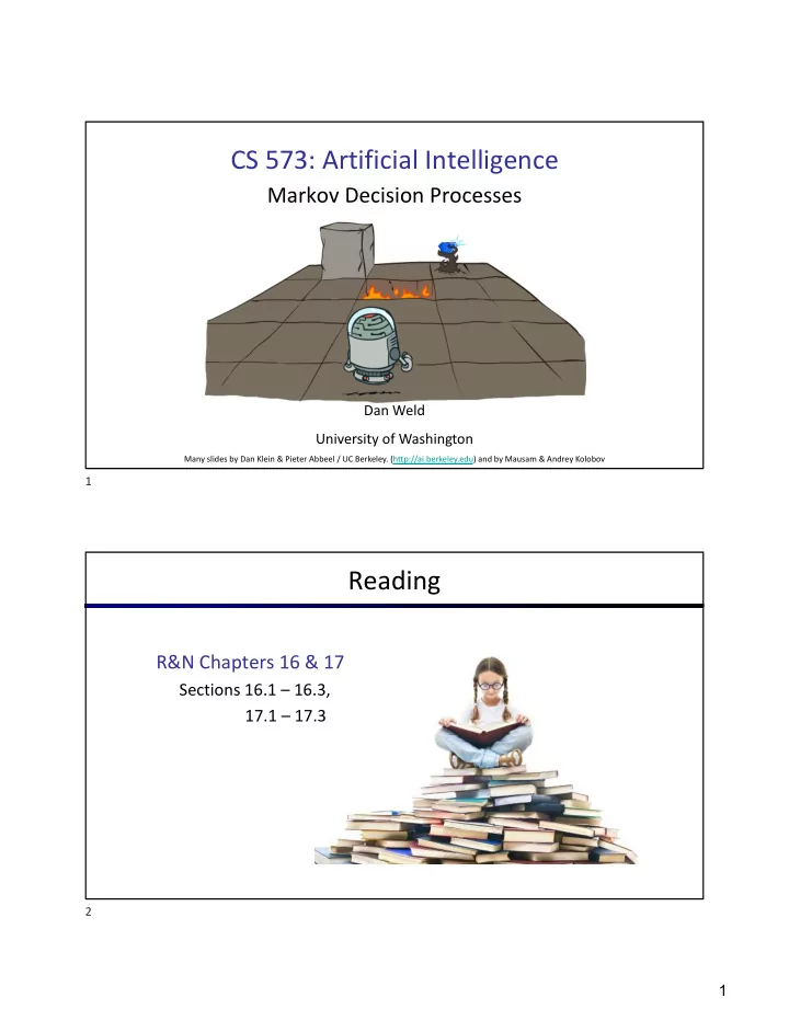

CS 573: Artificial Intelligence Markov Decision Processes Dan Weld University of Washington Many slides by Dan Klein & Pieter Abbeel / UC Berkeley. (http://ai.berkeley.edu) and by Mausam & Andrey Kolobov 1 Reading R&N Chapters 16 & 17 Sections 16.1 – 16.3, 17.1 – 17.3 2 1
Outline State Spaces Search Algorithms & Heuristics Adversarial Environments Stochastic Environments Expectimax Markov Decision Processes Value iteration Policy iteration Reinforcement Learning 4 Preferences & Utility Functions 6 2
Axioms of Rational Preferences 8 Axioms of Rational Preferences 9 3
Axioms of Rational Preferences 10 MEU Principle § Theorem [Ramsey, 1931; von Neumann & Morgenstern, 1944] § Given any preferences satisfying these constraints, there exists a real- valued function U such that: § I.e. values assigned by U preserve preferences of both prizes and lotteries! § Maximum expected utility (MEU) principle: § Choose the action that maximizes expected utility § Note: an agent can be entirely rational (consistent with MEU) without ever representing or manipulating utilities and probabilities § E.g., a lookup table for perfect tic-tac-toe, a reflex vacuum cleaner 11 4
Utility Scales § How Measure Human Utility? (e.g., what units)? § Micromorts: one-millionth chance of death, useful for paying to reduce product risks, etc. § QALYs: quality-adjusted life years, useful for medical decisions involving substantial risk § Maximize expected utility à § Behavior is invariant under positive linear transformation § WoLoG Normalized utilities: u + = 1.0, u - = 0.0 13 Human Utilities § Utilities map states to real numbers. Which numbers? § Standard approach to assessment (elicitation) of human utilities: § Compare a prize A to a standard lottery L p between § “best possible prize” u + with probability p § “worst possible catastrophe” u - with probability 1-p § Adjust lottery probability p until indifference: A ~ L p § Resulting p is a utility in [0,1] 0.999999 0.000001 Pay $30 No change Instant death 14 5
Money § Money does not behave as a utility function, but we can talk about the utility of having money (or being in debt) § Given a lottery L = [p, $X; (1-p), $Y] § The expected monetary value EMV(L) is p*X + (1-p)*Y § U(L) = p*U($X) + (1-p)*U($Y) § Typically, U(L) < U( EMV(L) ) § In this sense, people are risk-averse § When deep in debt, people are risk-prone 15 Example: Insurance Consider the lottery [0.5, $1M; 0.5, $0] § What is its expected monetary value? ($500K) § What is its certainty equivalent? § Monetary value acceptable in lieu of lottery § $400K for most people § Difference of $100K is the insurance premium § There’s an insurance industry because people will pay to reduce their risk § If everyone were risk-neutral, no insurance needed! § It’s win-win: you’d rather have the $400K and § The insurance company would rather have the lottery (why?) 16 6
Example: Grid World § A maze-like problem § The agent lives in a grid § Walls block the agent’s path § Noisy movement § Actions may not have intended effects § The agent receives `rewards’ on each time step § Small “living” reward each step (can be negative) § Big rewards come at the end (good or bad) § Goal: ~ maximize sum of rewards 19 Markov Decision Processes § An MDP is defined by: § A set of states s Î S § A set of actions a Î A § A transition function T(s, a, s’) § Probability that a from s leads to s’, i.e., P(s’| s, a) § Also called the model or the dynamics T(s 11 , E, … … T(s 31 , N, s 11 ) = 0 T is a Big Table! … T(s 31 , N, s 32 ) = 0.8 11 X 4 x 11 = 484 entries T(s 31 , N, s 21 ) = 0.1 T(s 31 , N, s 41 ) = 0.1 For now, we give this as input to the agent … 21 7
Markov Decision Processes § An MDP is defined by: § A set of states s Î S § A set of actions a Î A § A transition function T(s, a, s’) § Probability that a from s leads to s’, i.e., P(s’| s, a) § Also called the model or the dynamics § A reward function R(s, a, s’) … Cost of breathing R(s 32 , N, s 33 ) = -0.01 … R(s 32 , N, s 42 ) = -1.01 R is also a Big Table! … R(s 33 , E, s 43 ) = 0.99 For now, we also give this to the agent 22 Markov Decision Processes § An MDP is defined by: § A set of states s Î S § A set of actions a Î A § A transition function T(s, a, s’) § Probability that a from s leads to s’, i.e., P(s’| s, a) § Also called the model or the dynamics § A reward function R(s, a, s’) § Sometimes just R(s) or R(s’) … R(s 33 ) = -0.01 R(s 42 ) = -1.01 R(s 43 ) = 0.99 23 8
What is Markov about MDPs? § “Markov” generally means that given the present state, the future and the past are independent § For Markov decision processes, “Markov” means action outcomes depend only on the current state Andrey Markov (1856-1922) § This is just like search, where the successor function can only depend on the current state (not the history) 25 Input: MDP, Output: Policy § In deterministic single-agent search problems, we wanted an optimal plan, or sequence of actions, from start to a goal § For MDPs, want an optimal policy p *: S → A § A policy p gives an action for each state § An optimal policy is one that maximizes expected utility if followed § An explicit policy defines a reflex agent Optimal policy when R(s, a, s’) = -0.03 for all non-terminals s § Expectimax didn’t output an entire policy § It computed the action for a single state only 26 9
Optimal Policies R(s) = -0.01 R(s) = -0.03 Cost of breathing R(s) = -0.4 R(s) = -2.0 27 Another Example: Autonomous Driving (slightly simplified) 28 10
Example: Autonomous Driving § A robot car wants to travel far, quickly § Three states: Cool, Warm, Overheated § Two actions: Slow , Fast 0.5 +1 § Going faster gets double reward 1.0 Fast § Except when warm Slow -10 +1 0.5 Warm Slow Fast 0.5 +2 Cool 0.5 Overheated +1 1.0 +2 29 Example: Autonomous Driving S ? A ? T ? 0.5 +1 1.0 R ? Fast Slow -10 S 0 ? +1 0.5 Warm Slow Fast 0.5 +2 0.5 Cool Overheated +1 1.0 +2 30 11
Driving: Search Tree 2 2 1 2 1 1 2 1 2 2 1 -10 Two challenges for ExpectiMax: 1) Repeated states, 2) incremental reward (Great solutions coming soon) 31 Utilities of Sequences 32 12
Utilities of Sequences § What preferences should an agent have over reward sequences? § More or less? [1, 2, 2] or [2, 3, 4] [0, 0, 1] or [1, 0, 0] § Now or later? [1, 2, 3] or [3, 1, 1] § Harder… § Infinite sequences? [1, 2, 1, …] or [2, 1, 2, …] 33 Discounting § It’s reasonable to maximize the sum of rewards § It’s also reasonable to prefer rewards now to rewards later § One solution: values of rewards decay exponentially Worth Now Worth Next Step Worth In Two Steps 34 13
Discounting § How to discount? § Each time we descend a level, we multiply by the discount § Why discount? § Sooner rewards probably do have higher utility than later rewards § Also helps our algorithms converge § Example: discount of 0.5 § U([1,2,3]) = 1*1 + 0.5*2 + 0.25*3 = 2.75 § U([3,1,1]) = 1*3 + 0.5*1 + 0.25*1 = 3.75 § U([1,2,3]) < U([3,1,1]) 35 Quiz: Discounting § Given: § Actions: East, West, and Exit (only available in exit states a, e) § Transitions: deterministic § Quiz 1: For g = 1, what is the optimal policy? § Quiz 2: For g = 0.1, what is the optimal policy? § Quiz 3: For which g are West and East equally good when in state d? 36 14
Stationary Preferences § Theorem: if we assume stationary preferences: § Then: there are only two ways to define utilities § Additive utility: § Discounted utility: 37 Infinite Utilities?! § Problem: What if the game lasts forever? Do we get infinite rewards? § Solutions: 1. Discounting: use 0 < g < 1 Smaller g means smaller “horizon” – shorter term focus 2. Finite horizon: (similar to depth-limited search) Add utilities, but terminate episodes after a fixed T-steps lifetime Gives non-stationary policies ( p depends on time left)! 3. Absorbing state: guarantee that for every policy, a terminal state (like “overheated” for racing) will eventually be reached (eg. If every action has a non-zero chance of overheating) 38 15
Recap: Defining MDPs § Markov decision processes: s § Set of states S a § Start state s 0 § Set of actions A s, a § Transitions P(s’|s,a) (or T(s,a,s’)) s,a,s ’ § Rewards R(s,a,s’) (and discount g ) s ’ § MDP quantities so far: § Policy = Choice of action for each state § Utility = sum of (discounted) rewards 39 Solving MDPs § Value Iteration § Asynchronous VI § RTDP § Etc... § Policy Iteration § Reinforcement Learning 40 16
p * Specifies The Optimal Policy p * (s) = optimal action from state s 41 V* = Optimal Value Function The expected value (utility) of state s: V * (s) “expected utility starting in s & acting optimally forever” Equivalently: “expected value of s, following p * forever” 42 17
Q* The value (utility) of the q-state (s,a): Q * (s,a) “expected utility of 1) starting in state s 2) first taking action a 3) acting optimally (ala p * ) forever after that” Q*(s,a) = reward from executing a in s then ending in some s’ plus… discounted value of V*(s’) 43 The Bellman Equations How to be optimal: Step 1: Take best first action Step 2: Keep being optimal 44 18
Recommend
More recommend