CS 4100: Artificial Intelligence Bayes Nets: Sampling Jan-Willem - PDF document

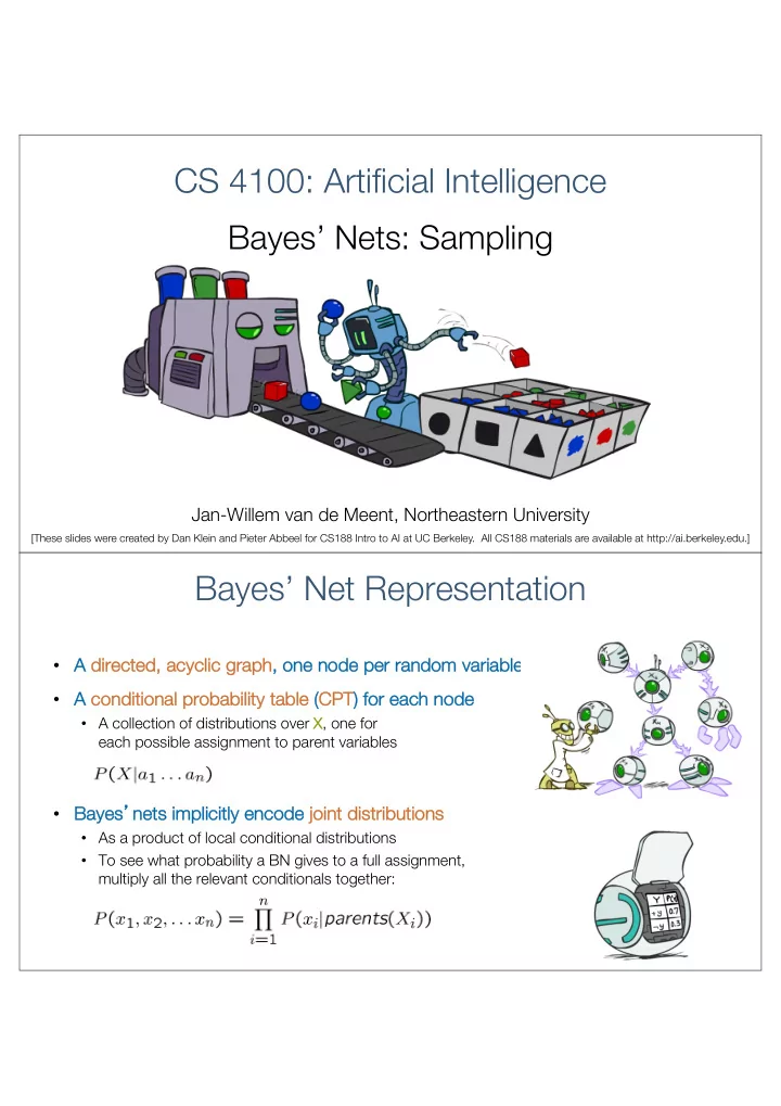
CS 4100: Artificial Intelligence Bayes’ Nets: Sampling Jan-Willem van de Meent, Northeastern University [These slides were created by Dan Klein and Pieter Abbeel for CS188 Intro to AI at UC Berkeley. All CS188 materials are available at http://ai.berkeley.edu.] Bayes’ Net Representation • A A di directed, d, acyclic graph ph, o , one n node p per r random v variable • A A co conditional al probab ability tab able (CP CPT) ) for each node de • A collection of distributions over X , one for each possible assignment to parent variables • Ba Bayes ’ ne nets implicitly enc ncode jo join int dis istrib ributio ions • As a product of local conditional distributions • To see what probability a BN gives to a full assignment, multiply all the relevant conditionals together:

Variable Elimination • Interleave ve jo join inin ing and and marginalizi zing • d k entries s computed for a factor ove ver k variables va s with domain si size zes s d … • Or Orde dering of elimination of hidden va variables s … can can af affect ect si size ze of factors s ge generate ted • Worst st case se: running time exp xponential in the si in size ze of the Baye yes’ s’ net Approximate Inference: Sampling

Sampling • Sampling is a lot like ke repeated simulation • Why Why sampl ple? • Predicting the weather, basketball games, … • Re Reinforcement Learning: Can approximate (q-)values even when you don’t know the transition function • Ba Basic idea • In Inference: : getting a sample is faster than Draw N samples from a sampling distribution S • Dr computing the right answer (e.g. with Compute an approximate posterior probability variable elimination) • Co • Show this co ges to the true probability P conver verges Sampling • Example u u = 0.83 • Sampling from give ven dist stribution C P(C) • St Step p 1: Get sample u from uniform distribution over [0 [0, 1) 0 0.6 0.7 1.0 red 0.6 • E.g. ra random() m() in python green 0.1 • St Step p 2: Convert this sample u into blue 0.3 an outcome for the given distribution by having each target outcome associated with a sub-interval of [0,1) with sub-interval size equal to [0 • If ra random() returns u = = 0.83 , probability of the outcome then our sample is C = = blue • E.g, after sampling 8 times:

Sampling in Bayes’ Nets • Pr Prior ior Sa Samp mplin ling • Re Rejecti tion Sampling • Like kelihood Weighting • Gi Gibbs Sampling Prior Sampling

Prior Sampling +c 0.5 -c 0.5 Cloudy Cloudy +c +s 0.1 +c +r 0.8 -s 0.9 -r 0.2 +s 0.5 +r 0.2 -c -c Sprinkler Sprinkler Rain Rain -s 0.5 -r 0.8 Samples: WetGrass WetGrass +r +w 0.99 +s +c, -s, +r, +w -w 0.01 +w 0.90 -r -c, +s, -r, +w -w 0.10 … +r +w 0.90 -s -w 0.10 +w 0.01 -r -w 0.99 Prior Sampling • For For i = 1 , 2 , …, n • Sa Sampl ple x i fr from P( P(X i | Parents( s(X i )) )) • Re Return (x (x 1 , x , x 2 , …, …, x n )

Prior Sampling • This s process ss generates s sa samples s with pr proba babi bility ty: … i.e … .e. th . the B BN’s s joint probability • Let the number of sa samples s of an eve vent be • Then Then • i.e., the sa sampling procedure is s consi sist stent* (different from consi sist stent heurist stic, or arc consi sist stency) y) Example • We We’ll ll dr draw w a ba batch of sa samples f s from t the B BN: +c +c, -s, +r +r, +w +w C +c, +s +c +s, +r +r, +w +w S R -c, +s +s, +r +r, -w +c +c, -s, +r +r, +w +w W -c, c, -s, s, -r, +w +w • If we want to kn know P( P(W) Count outcomes <+ • Co <+w: 4 : 4, , -w: 1 : 1> lize to get P(W) = • No Normaliz = <+w <+w: 0 : 0.8 .8, , -w: 0 : 0.2 .2> • Estimate will get closer to the true distribution with more samples • Can estimate anything else, too • What about P(C | +w +w) ? P( P(C | +r, r, +w +w) ? P( P(C | -r, r, -w) ? • Fa Fast st: can use fewer samples if less time (what’s the drawback?)

Rejection Sampling Rejection Sampling • Le Let’ t’s s sa say y we want P( P(C) • No point keeping all samples around C • Just tally counts of C as we go S R W • Le Let’ t’s s sa say y we want P( P(C | +s) idea: tally C outcomes, but ignore • Sa Same me id +c, -s, +r +c +r, +w +w (reject) samples which don’t have S= S=+s +c, +s +c +s, +r +r, +w +w • This is called re reje jectio ion samplin ling -c, +s +s, +r +r, -w +c +c, -s, +r +r, +w +w • It is also consistent for conditional probabilities -c, c, -s, s, -r, +w +w (i.e., correct in the limit of large N )

Rejection Sampling • In Input: t: evidence assignments • For For i = 1, 2, …, …, n • Sa Sample mple x i fr from om P(X P(X i | Parents( s(X i )) )) • If If x i not consi sist stent with evi vidence • Re Reje ject: Return – no sample is generated in this cycle • Re Return (x (x 1 , x , x 2 , …, …, x n ) Likelihood Weighting

<latexit sha1_base64="91+0FuZ923Dcgnlovm9ic1E65zk=">AHK3icfZVb9MwFMe9AWU28YeanokIaIqmQd3eBp2pjG2ViF6mpJidx21Dngu107Sx/Fl7hgU/DE4hXvgd2EiCJwxylsc75nb+P3WPbibFPmWl+X1q+cfNW4/bKnebde/cfPFxde3RKo4S46MSNcETOHUgR9kN0wnyG0XlMEAwcjM6c6YHyn80QoX4UvmeLGA0DOA79ke9CJk0Xq+v9zQOjdyA9rPadG6/nls4vVtkx09bSO1beae+BrPUv1hrA9iI3CVDIXAwpHVhmzIYcEua7GImnVAUQ3cKx2guyEMEB3yNHvRajafFvw8RJfxnKE5EzX2ALKJaBb1OAxoZq0YR1HIaNmKodSli6BsdYKy4gDN4io9L0PCWVONBcqRQ+N5BqnOXPwQkS/PhoX3DT6HUNa2tHVBmCvByxdk1DPhoxJgiFObO7bVi93RoTkiM0T/KVJzKuEi9hmTaz0E3WExlWp1ez5D/lWGmb7cr9Ij9dBYZb+XYdfyxmtEfeTNVz8Je1MAHCxiWxdVr/Yc+ypaikLt5rfpbAsMxKmZTmLBKXi4QbJm3CgIYOhxe4ZcMbCG3EYhTQhSNcNtJ8KeLAj54W1LCKEFZSEyNvVL0aIXzSAW3DZk0AgjV5UK37Axgh5l0YawX1UD5qI8/IzP0GLzEJjFhpzpTFXGjPRGBsxWDPHpAwmVaGPFSE2SXWqMriCYXkIeTUcq8pBbcRBYknvrb2kIwDqNYzihGBLCLqULn02QT7gc8oz/1Cj/LD6OkvzrYSUh9es4/FBopOvgtGRkr7zN0vIpo8TULXDasgx0chsw9Swsc7mJ0MN7C40ON23NWik6+abUMHpnfFStd7fG0LvnG51rG6n+267vbef3x4r4DF4AjaBXbAHngD+uAEuGABPoHP4Evja+Nb40fjZ4YuL+Ux6DUGr9+A/T9jb4=</latexit> Likelihood Weighting • Pr Problem m with rejection samp mpling: • Id Idea: ea: fi fix ev eviden ence ce an and sa sample t the r rest st • If evidence is unlikely, rejects lots of samples • Pr Probl blem: sample distribution not consistent! • Evidence not exploited as you sample • So Solution: Assign a we weig ight by according to probability of evidence given parents • Consider P( P( Sh Shape pe | bl blue ) pyramid, blue pyramid, green pyramid, blue pyramid, red sphere, blue Shape Color Shape Color sphere, blue cube, blue cube, red sphere, blue sphere, green Likelihood Weighting Ex Examp mple: P ( C, R | + s, + w ) +c 0.5 -c 0.5 Cloudy Cloudy +s 0.1 +r 0.8 +c +c -s 0.9 -r 0.2 -c +s 0.5 -c +r 0.2 Sprinkler Rain Rain -s 0.5 -r 0.8 Samples: WetGrass WetGrass +w 0.99 +r +s +c, +s, +r, +w -w 0.01 -r +w 0.90 … -w 0.10 +w 0.90 +r -s -w 0.10 -r +w 0.01 In Intuition: As Assign higher w w to to “good” samples -w 0.99 (i.e. samples with high probability for evidence)

Likelihood Weighting • In Input: t: evidence assignment • w w = 1. 1.0 • for or i = 1 , 2 , …, n • if X i is s an evi vidence va variable • X i = x i (from evidence) • w w = w * P( P(x i | Parents( s(X i )) )) • else se • Sam Sampl ple x i fro from P( P(X i | Parents( s(X i )) )) • Ret etur urn n (x (x 1 , x , x 2 , …, …, x n ) , w Likelihood Weighting • Sampling dist stribution if z sa sampled and e fixe xed evi vidence Cloudy C S R • Now, sa samples s have ve we weig ights ts W • Together, weighted sa sampling dist stribution is s consi sist stent

Ex Exerc rcise: Sampling ng fro rom p(B p(B, E, A | +j, j, +m) ) in in Ala larm Netwo twork B P(B) E P(E) B E A P(A|B,E) B E +b +e +a 0.95 +b 0.001 +e 0.002 +b +e -a 0.05 -b 0.999 -e 0.998 +b -e +a 0.94 A +b -e -a 0.06 A J P(J|A) A M P(M|A) -b +e +a 0.29 +a +j 0.9 +a +m 0.7 -b +e -a 0.71 +a -j 0.1 +a -m 0.3 J M -b -e +a 0.001 -a +j 0.05 -a +m 0.01 -b -e -a 0.999 -a -j 0.95 -a -m 0.99 1. What is the probability of p( p(-b, b, -e, e, -a) a) ? 2. What weight w w will likelihood weighting assign to a sample -b, b,-e, e, -a ? 3. What weight w w will likelihood weighting assign to a sample -b,-e, + , +a ? 4. Will rejection sampling reject more or less than 99.9% of the samples? Likelihood Weighting • The The Good ood: We take • Like kelihood weighting doesn’t t solve all our r problems ke evidence in into to account t as as we we gen ener erat ate e do down wnstr tream sa samples Evidence influences samples for do down wnstr tream • E.g. here, W’ W’s value will get picked based on variables, but not up upst stream ones • the evidence values of S , R (were aren’t more likely to sample a “good” value for C C that matches the evidence) • More of our samples will reflect the state of the world suggested by the evidence • We would like ke to consider evidence when we sam sample every var ariab able e (lead eads s to o Gib Gibbs samplin ling) C S R W