CS 331: Artificial Intelligence Probability I Thanks to Andrew - PDF document

CS 331: Artificial Intelligence Probability I Thanks to Andrew Moore for some course material 1 Dealing with Uncertainty • We want to get to the point where we can reason with uncertainty • This will require using probability e.g. probability that it will rain today is 0.99 • We will review the fundamentals of probability 2 1

Outline 1. Random variables 2. Probability Random Variables • The basic element of probability is the random variable • Think of the random variable as an event with some degree of uncertainty as to whether that event occurs • Random variables have a domain of values it can take on 4 2

Random Variables Example: • ProfLate is a random variable for whether your prof will be late to class or not • The domain of ProfLate is { true , false} – ProfLate = true : proposition that prof will be late to class – ProfLate = false : proposition that prof will not be late to class 5 Random Variables Example: • ProfLate is a random variable for whether your prof will be late to class or not • The domain of ProfLate is < true , false > – ProfLate = true : proposition that prof will be late to class You can assign some degree of – ProfLate = false : proposition that prof belief to this proposition e.g. will not be late to class P(ProfLate = true) = 0.9 6 3

Random Variables Example: • ProfLate is a random variable for whether your prof will be late to class or not • The domain of ProfLate is < true , false > – ProfLate = true : proposition that prof will be late to class – ProfLate = false : proposition that prof will not be late to class And to this one e.g. P(ProfLate = false) = 0.1 7 Random Variables • We will refer to random variables with capitalized names e.g. X , Y , ProfLate • We will refer to names of values with lower case names e.g. x , y , proflate • This means you may see a statement like ProfLate = proflate – This means the random variable ProfLate takes the value proflate (which can be true or false ) • Shorthand notation : ProfLate = true is the same as proflate and ProfLate = false is the same as ¬ proflate 8 4

Random Variables 3 types of random variables: 1. Boolean random variables 2. Discrete random variables 3. Continuous random variables Boolean Random Variables • Take the values true or false • E.g. Let A be a Boolean random variable – P(A = false) = 0.9 – P(A = true) = 0.1 10 5

Discrete Random Variables Allowed to taken on a finite number of values e.g. • P(DrinkSize=small) = 0.1 • P(DrinkSize=medium) = 0.2 • P(DrinkSize=large) = 0.7 Discrete Random Variables Values of the domain must be: • Mutually Exclusive i.e. P( A = v i AND A = v j ) = 0 if i  j This means, for instance, that you can’t have a drink that is both small and medium • Exhaustive i.e. P(A = v 1 OR A = v 2 OR ... OR A = v k ) = 1 This means that a drink can only be either small , medium or large . There isn’t an extra large. 6

Discrete Random Variables Values of the domain must be: • Mutually Exclusive i.e. P( A = v i AND A = v j ) = 0 if i  j This means, for instance, that you can’t have a The AND here means intersection i.e. (A = v i )  (A = v j ) drink that is both Small and Medium • Exhaustive i.e. P(A = v 1 OR A = v 2 OR ... OR A = v k ) = 1 This means that a drink can only be either small , The OR here means union i.e. (A = v 1 )  medium or large . There isn’t an extra large (A = v 2 )  ...  (A = v k ) Discrete Random Variables • Since we now have multi-valued discrete random variables we can’t write P(a) or P(¬a) anymore • We have to write P(A = v i ) where v i = a value in { v 1 , v 2 , …, v k } 14 7

Continuous Random Variables • Can take values from the real numbers • E.g. They can take values from [0, 1] • Note: We will primarily be dealing with discrete random variables • (The next slide is just to provide a little bit of information about continuous random variables) 15 Probability Density Functions Discrete random variables have probability distributions: 1.0 P( A ) a ¬a Continuous random variables have probability density functions e.g: P( X ) P( X ) X X 8

Probabilities • We will write P(A=true) as “the fraction of possible worlds in which A is true” • We can debate the philosophical implications of this for the next 4 hours • But we won’t Probabilities • We will sometimes talk about the probabilities of all possible values of a random variable • Instead of writing – P(A=false) = 0.25 – P(A=true) = 0.75 • We will write P ( A ) = (0.25, 0.75) Note the boldface! 18 9

Visualizing A Event space of all possible P( a ) = Area of Worlds in which worlds A is true reddish oval Its area is 1 Worlds in which A is false 19 The Axioms of Probability • 0  P( a )  1 • P( true ) = 1 • P( false ) = 0 • P( a OR b ) = P( a ) + P( b ) - P( a AND b ) The logical OR is equivalent to set The logical AND is equivalent to union  . set intersection (  ). Sometimes, I’ll write it as P(a, b) These axioms are often called Kolmogorov’s axioms in honor of the Russian mathematician Andrei Kolmogorov 20 10

Interpreting the axioms 0  P( a )  = 1 • • P( true ) = 1 • P( false ) = 0 • P( a OR b ) = P( a ) + P( b ) - P( a, b ) The area of P( a) can’t get any smaller than 0 And a zero area would mean that there is no world in which a is not false 21 Interpreting the axioms 0  P( a )  1 • • P( true ) = 1 • P( false ) = 0 • P( a OR b ) = P( a ) + P( b ) - P( a, b ) The area of P( a) can’t get any bigger than 1 And an area of 1 would mean all worlds will have a is true 22 11

Interpreting the axioms 0  P( a )  1 • • P( true ) = 1 • P( false ) = 0 • P( a OR b ) = P( a ) + P( b ) - P( a, b ) P( a, b ) [The purple area] a b P( a OR b ) [the area of both circles] 23 Prior Probability • We can consider P(A) as the unconditional or prior probability – E.g. P(ProfLate = true) = 1.0 • It is the probability of event A in the absence of any other information • If we get new information that affects A , we can reason with the conditional probability of A given the new information. 24 12

Conditional Probability • P( A | B ) = Fraction of worlds in which B is true that also have A true • Read this as: “Probability of A conditioned on B ” • Prior probability P( A ) is a special case of the conditional probability P( A | ) conditioned on no evidence 25 Conditional Probability Example H = “Have a headache” F = “Coming down with F Flu” P( H ) = 1/10 P( F ) = 1/40 P( H | F ) = 1/2 H “Headaches are rare and flu is rarer, but if you’re coming down with ‘flu there’s a 50 - 50 chance you’ll have a headache.” 26 13

Conditional Probability P( H | F ) = Fraction of flu-inflicted F worlds in which you have a headache # worlds with flu and headache  # worlds with flu H Area of " H and F" region  Area of " F" region P(H, F)  P(F) H = “Have a headache” F = “Coming down with Flu” P( H ) = 1/10 P( F ) = 1/40 27 P( H | F ) = 1/2 Definition of Conditional Probability ( , ) P A B  ( | ) P A B ( ) P B Corollary: The Chain Rule (aka The Product Rule)  ( , ) ( | ) ( ) P A B P A B P B 28 14

Important Note    ( | ) ( | ) 1 P A B P A B But:    ( | ) ( | ) does not always 1 P A B P A B 29 The Joint Probability Distribution • P( A , B ) is called the joint probability distribution of A and B • It captures the probabilities of all combinations of the values of a set of random variables 30 15

The Joint Probability Distribution • For example, if A and B are Boolean random variables, then P( A , B ) could be specified as: P( A = false , B = false ) 0.25 P( A = false , B = true ) 0.25 P( A = true , B = false ) 0.25 P( A = true , B = true ) 0.25 31 The Joint Probability Distribution • Now suppose we have the random variables: – Drink = { coke , sprite } – Size = { small , medium, large } • The joint probability distribution for P( Drink , Size ) could look like: P( Drink = coke , Size = small ) 0.1 P( Drink = coke , Size = medium ) 0.1 P( Drink = coke , Size = large ) 0.3 P( Drink = sprite , Size = small ) 0.1 P( Drink = sprite , Size = medium ) 0.2 P( Drink = sprite , Size = large ) 0.2 32 16

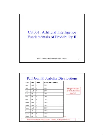
Full Joint Probability Distribution • Suppose you have the complete set of random variables used to describe the world • A joint probability distribution that covers this complete set is called the full joint probability distribution • Is a complete specification of one’s uncertainty about the world in question • Very powerful: Can be used to answer any probabilistic query 33 17