CS 188: Artificial Intelligence Spring 2006 Lecture 5: Robot Motion - - PDF document

1

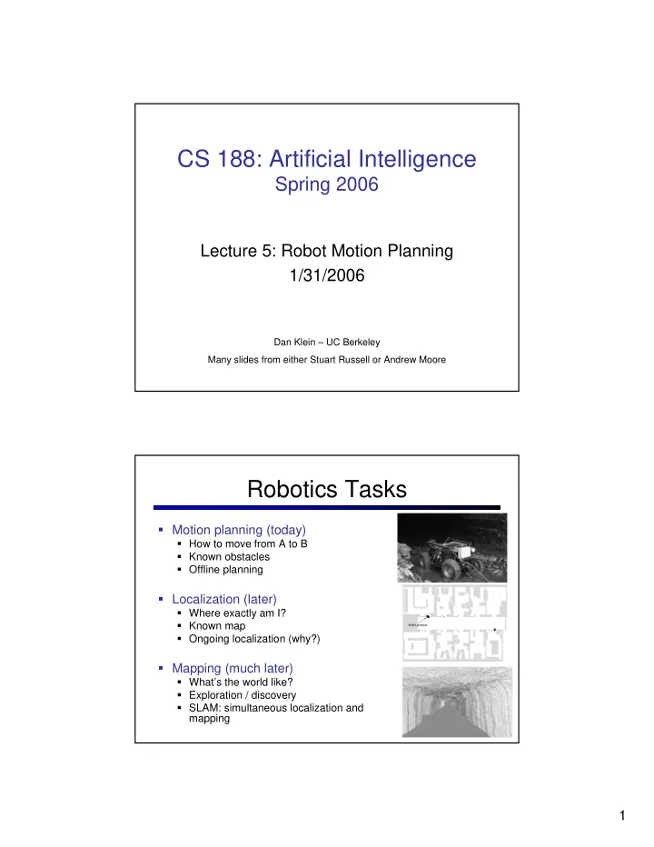
CS 188: Artificial Intelligence

Spring 2006

Lecture 5: Robot Motion Planning 1/31/2006

Dan Klein – UC Berkeley Many slides from either Stuart Russell or Andrew Moore

Robotics Tasks

Motion planning (today)

How to move from A to B Known obstacles Offline planning

Localization (later)

Where exactly am I? Known map Ongoing localization (why?)

Mapping (much later)

What’s the world like? Exploration / discovery SLAM: simultaneous localization and mapping

2

Mobile Robots

High-level objectives: move robots around obstacles Low-level: fine motor control to achieve motion Why is this hard?

Start Configuration Immovable Obstacles Goal Configuration

Manipulator Robots

High-level goals: reconfigure environment Low-level: move from configuration A to B (point-to-point motion)

Why is this already hard?

Also: compliant motion

3

Sensors and Effectors

Sensors vs. Percepts

Agent programs receive percepts Agent bodies have sensors Includes proprioceptive sensors Real world: sensors break, give noisy answers, miscalibrate, etc.

Effectors vs. Actuators

Agent programs have actuators (control lines) Agent bodies have effectors (gears and motors) Real-world: wheels slip, motors fail, etc.

Degrees of Freedom

2 DOFs 3 DOFs Question: How many DOFs for a polyhedron free-flying in 3D space?

The degrees of freedom are the numbers required to specify a robot’s configuration Positional DOFs:

(x, y, z) of free-flying robot direction robot is facing

Effector DOFs

Arm angle Wing position

Static state: robot shape and position Dynamic state: derivatives of static DOFs (why have these?)

4

Example

How many DOFs?

What are the natural coordinates for specifying the robot’s configuration? These are the configuration space coordinates What are the natural coordinates for specifying the effector tip’s position? These are the work space coordinates

Example

How many DOFs?

How does this compare to your arm? How many are required for arbitrary positioning of end-effector?

5

Holonomicity

Holonomic robots control all their DOFs (e.g. manipulator arms)

Easier to control Harder to build

Non-holonomic robots do not directly control all DOFs (e.g. a car)

Configuration Space

Workspace:

The world’s (x, y) system Obstacles specified here

Configuration space

The robot’s state Planning happens here

6

Kinematics

Kinematics

The mapping from configurations to workspace coordinates Generally involves some trigonometry Usually pretty easy

Inverse Kinematics

The inverse: effector positions to configurations Usually non-unique (why?)

Forward kinematics

Configuration Space

• Configuration space

Just a coordinate system Not all points are reachable / legal

• Legal configurations:

No collisions No self-intersection

7

Obstacles in C-Space

What / where are the obstacles? Remaining space is free space

More Obstacles

8

Topology

You very quickly get into issues of topology:

Point robot in 3D: R3 Directional robot with fixed position in 3D: SO(3) Two rotational-jointed robot in 2D: S1xS1

For the present purposes, we’ll basically ignore these issues In practice, you have to deal with it properly

Example: 2D Polygons

Workspace Configuration Space

9

Example: Rotation Example: A Less Simple Arm

10

Summary

Degrees of freedom Legal robot configurations form configuration space Obstacles have complex images in c- space

Motion as Search

Motion planning as path-finding problem

Problem: configuration space is continuous Problem: under-constrained motion Problem: configuration space can be complex

Why are there two paths from 1 to 2?

11

Decomposition Methods

Break c-space into discrete regions Solve as a discrete problem

Exact Decomposition?

With polygon obstacles: decompose exactly Problems?

Doesn’t scale at all Doesn’t work with complex, curved obstacles

12

Approximate Decomposition

Break c-space into a grid

Search (A*, etc) What can go wrong? If no path found, can subdivide and repeat

Problems?

Still scales poorly Incomplete* Wiggly paths

S G

Hierarchical Decomposition

But:

Not optimal Not complete Still hopeless above a small number of dimensions

Actually used in practical systems

13

Skeletonization Methods

Decomposition methods turn configuration space into a grid Skeletonization methods turn it into a set of points, with preset linear path between them

Visibility Graphs

Shortest paths:

No obstacles: straight line Otherwise: will go from vertex to vertex Fairly obvious, but somewhat awkward to prove

Visibility methods:

All free vertex-to-vertex lines (visibility graph) Search using, e.g. A* Can be done in O(n3) easily, O(n2log(n)) less easily

Problems?

Bang, screech! Not robust to control errors Wrong kind of optimality?

qstart qgoal qstart

14

Voronoi Decomposition

Voronoi regions: points colored by closest obstacle Voronoi diagram: borders between regions

Can be calculated efficiently for points (and polygons) in 2D In higher dimensions, some approximation methods

R G B Y

Voronoi Decomposition

Algorithm:

Compute the Voronoi diagram

• f the configuration space

Compute shortest path (line) from start to closest point on Voronoi diagram Compute shortest path (line) from goal to closest point on Voronoi diagram. Compute shortest path from start to goal along Voronoi diagram

Problems:

Hard over 2D, hard with complex obstacles Can do weird things:

15

Probabilistic Roadmaps

Idea: just pick random points as nodes in a visibility graph This gives probabilistic roadmaps

Very successful in practice Lets you add points where you need them If insufficient points, incomplete,

• r weird paths

Roadmap Example

16

Potential Field Methods

So far: implicit preference for short paths Rational agent should balance distance with risk! Idea: introduce cost for being close to an

• bstacle

Can do this with discrete methods (how?) Usually most natural with continuous methods

Potential Fields

Cost for:

Being far from goal Being near an

• bstacle

Go downhill What could go wrong?

17

Potential Field Methods

SIMPLE MOTION PLANNER: Gradient descent on u

( ) ( ) ( ) ( ) ( )

( )

( )

∑

+ = − = = ⎟ ⎠ ⎞ ⎜ ⎝ ⎛ = ⎟ ⎠ ⎞ ⎜ ⎝ ⎛ → → ℜ → ⎟ ⎠ ⎞ ⎜ ⎝ ⎛

2 2 ~ ~ ~ ~ ~ ~

1 2 1 2 1 : definition Preferred :

• f

definition One

• bstacle

nearest to from distance goal to from distance Write goal the towards move you as small

• bstacle

an towards move you as huge Such that ions Configurat : function a Define q d q d q u q d q d q u u q q d q q q d u u u q u

i g g i i g

η

Local Search Methods

Queue-based algorithms keep fallback

• ptions (backtracking)

Local search: improve what you have until you can’t make it better Generally much more efficient (but incomplete)

18

Gradient Methods

How to deal with continous (therefore infinite) state spaces? Discretization: bucket ranges of values

E.g. force integral coordinates

Continuous optimization

E.g. gradient ascent (or descent)

Image from vias.org

Hill Climbing

Simple, general idea:

Start wherever Always choose the best neighbor If no neighbors have better scores than current, quit

Why can this be a terrible idea?

Complete? Optimal?

What’s good about it?

19

Hill Climbing Diagram

Random restarts? Random sideways steps?