Critical points of smooth Gaussian random fields Jonathan Taylor - PowerPoint PPT Presentation
Critical points of smooth Gaussian random fields Jonathan Taylor (Stanford) November 11, 2014 Two Stages A model for random sets. Critical points: Kac-Rice formula. Tube formulae. Gaussian integral geometry. Selective
Critical points of smooth Gaussian random fields Jonathan Taylor (Stanford) November 11, 2014
Two Stages • A model for random sets. • Critical points: Kac-Rice formula. • Tube formulae. • Gaussian integral geometry. • Selective inference for critical points.
References • Most of what I am going to say today can be found in Random Fields and Geometry. • Results built on top of earlier work of: • Robert Adler • Iain Johnstone • Satoshi Kuriki • David Siegmund • Jiayang Sun • Akimichi Takemura • Keith Worsley • Weyl, Hotelling • Last part of talk related to selective inference (See arxiv.org/1308.3020)
A model for random sets • Our basic building blocks are R -valued Gaussian random fields on some n -dimensional manifold M (maybe with corners). • We think of M as fixed, not large volume / high frequency properties. • The only asymptotic we look at is excursion above a high level. • For most of the talk, we will assume: • E ( f t ) = 0 . • E ( f 2 t ) = 1 . • R ( t, s ) = E ( f t · f s ) . • (Put canonical picture / example on blackboard) • Is Gaussian necessary? • Only when we want to do some explicit computations. • Heavy-tailed can of course have different behavior.
Excursion above 0
Excursion above 1
Excursion above 1.5
Excursion above 2
Excursion above 2.5
Excursion above 3
Why care? • Integral geometric properties tell a nice geometric story. • Each component of the excursion set contains a critical point of f . • By Morse Theory, the Euler characteristic can be expressed in terms of critical points of f | f − 1 [ u + ∞ ) . . . • Critical points / values are of fundamental importance here. • One part of the story: for large u � � M ∩ f − 1 [ u, + ∞ ) � � �� E χ ≈ P sup f t ≥ u . t ∈ M
Statistical motivation • Signal detection in smooth noise. A natural test statistic for 1-sparse means H 0 : µ ≡ 0 , H a : µ ( · ) = α · R ( t 0 , · ) . • Nonregular likelihood ratio / score tests. Limiting distribution is often of the form max( f t , 0) 2 . sup t ∈ M
Kac-Rice formula • A fundamental tool for counting zeros. • Kac was interested in number of zeros of random polynomials. • Rice was interested in the number of upcrossings of a process above a level. • Suppose h : M → R n is sufficiently smooth and non-degenerate and g is continuous E (# { t ∈ M : h t = 0 , g t ∈ O } ) � � � � � = E 1 { g t ∈ O } · | Jh t | � h t = 0 φ h t (0) dt. � M
Kac-Rice formula • With a little imagination, this is roughly the same as � � � � � = � E F ( g t ) E F ( g t ) · | Jh ( t ) | � h t = 0 φ h t (0) dt � M t ∈ M : h t =0 for reasonable functions F : R → R .
Rough proof of Kac-Rice 1 � 1 [ u − ǫ,u + ǫ ] ( h ( t )) | h ′ ( t ) | dt 2 = lim 2 ǫ ǫ ↓ 0 [0 ,T ]
Rough proof of Kac-Rice Interchange ǫ ↓ 0 and expectation. . .
Tail probability • Applying Kac-Rice to local maxima: � � � # { t ∈ M : ∇ f t = 0 , f t ≥ u, ∇ 2 f t < 0 } � f t ≥ u ≤ E P sup t ∈ M � � � � � det( −∇ 2 f t )1 { f t ≥ u, ∇ 2 f t < 0 } = E � ∇ f t = 0 � M φ ∇ f t (0) dt � M n = t (1 { f t ≥ u } ) dt M • Above, � � � t ( h ) def M j h · det( −∇ 2 f t )1 { index ( ∇ 2 f t )= j } � = E � ∇ f t = 0 φ ∇ f t (0) �
Tail probability • The EC heuristic: n u →∞ M j � M n t (1 { f t ≥ u } ) ≈ t (1 { f t ≥ u } ) . j =0 • Morse’s theorem, followed by integration over M yields n � M j M ∩ f − 1 [ u, + ∞ ) � � � �� E χ = t (1 { f t ≥ u } ) dt M j =0
What does this tell you? • Let M be a 2-manifold without boundary, then = 1 f − 1 [0 , + ∞ ) � � �� E χ 2 χ ( M ) . • If we allow boundary, then = 1 2 χ ( M ) + 1 f − 1 [0 , + ∞ ) � � �� E χ 2 π | ∂M | . • Lengths and areas are computed with respect to a Riemannian metric from f : g ( X t , Y t ) = E ( X t f · Y t f ) .
Expected EC is computable • The EC stands out as being explicitly computable in wide generality. (Here and on last slide is where we use our centered Gaussian constant variance assumption) • Specifically, define � 1 − Φ( u ) j = 0 ρ j ( u ) = H j − 1 ( u ) e − u 2 / 2 (2 π ) ( j +1) / 2 j ≥ 1 • Then, n M ∩ f − 1 [ u, + ∞ ) � � � �� L j ( M ) ρ j ( u ) . E χ = j =0
How good is this approximation? • The expected EC heuristic does not assume Gaussianity (though calculations would be difficult otherwise) . • However, if f is Gaussian and as assumed here, a careful application of Kac-Rice yields � � � ��� � M ∩ f − 1 [ u, + ∞ ) � � � Error ( u ) = � P sup f t ≥ u − E χ � � � t ∈ M � � � � − u 2 / 2 1 1+ u →∞ σ 2 = O exp e c ( f,M ) • Error is roughly the cost of having two critical points above the level u .
Tube formulae • For small r , the functionals L j ( M ) are implicitly defined by Steiner-Weyl formula for r ≤ r c ( M ) k � x ∈ R k : d ( x, M ) ≤ r � � ω k − j r k − j L j ( M ) H k = j =0 • The quantity σ 2 c ( f, M ) is completely analogous to the critical radius of embedding of M in H f , the RKHS of f : M ∋ t �→ R ( t, · ) ∈ S ( H f ) .
The cube H 3 ( Tube ([0 , a ] × [0 , b ] × [0 , c ] , r )) = abc + 2 r · ( ab + bc + ac ) + ( πr 2 ) · ( a + b + c ) + 4 πr 3 3
How to compute volume of a tube t + r · η t t
The Jacobean • Most of the work (and all of the local information) is encoded in the Jacobean of ( t, η t ) �→ t + r · η t , � η � 2 = 1 This is what Weyl said anyone decent student of calculus could do. • Some careful thought and / or more calculus shows that det( −∇ 2 f t ) has a very similar structure to the above Jacobean.
Gaussian Kinematic Formula • Let f = ( f 1 , . . . , f k ) be made of IID copies of our original Gaussian field. • Consider the additive functional on R k that takes a rejection region M ∩ f − 1 D � � �� D �→ E χ . • For D that are rare under the marginal distribution ( γ k ∼ N (0 , I k × k ) ) the expected EC heuristic says M ∩ f − 1 D M ∩ f − 1 D � = ∅ � � �� � � E χ ≈ P . • How is M involved? (We suspect through L j ( M ) .) • How is D involved?
T random field
A simple cone The rejection region for a t statistic x 1 T ( x 1 , x 2 , x 3 ) = . � ( x 2 2 + x 2 3 ) / 2
Inverse image
Gaussian Kinematic Formula j on R k by • Define additive functionals M γ √ 2 πr ) j ( � y ∈ R k : d ( y, D ) ≤ r � M γ k � γ k = j ( D ) j ! j ≥ 0 • Then, the Gaussian Kinematic Formula asserts n L j ( M ) M γ k χ ( M ∩ f − 1 D ) � � � E = j ( D ) . j =0
Gaussian Kinematic Formula • Why do M γ k arise? Not clear beyond direct calculation. j • Can be proved by direct calculation with Kac-Rice. • Alternate proof based on classical Kinematic Fundamental Formula on √ � x ∈ R N : � x � 2 = � N ( R N ) = S √ N , N → ∞ . • Both proofs involve recognizing an integral as a coefficient in Gaussian tube expansion. • Because many canonical statistics are based on distance, it turns out there are perhaps more explicit examples of Gaussian tube formulae than Steiner . . . • Instead of examples I want to return to selective inference . . .
Selective inference • The measures M j t , suitably normalized, can be interpreted as a type of Palm distribution / Slepian model. • Define the normalized measures h ) = M j t (˜ h ) Q j t (˜ . M j t (1) • Formally, by Kac-Rice h �→ Q j t ( h ( f t )) determines the law of f t given t is a critical point of f with index j .
Selective inference • Can derive tests of H 0 : E ( f t ) ≡ 0 based on � � t ∗ = argmax t ∈ M f t . � sup f t � t ∈ M • Or selective tests of H 0 : f t ∗ = 0 . • Let’s take a closer look at the structure of such a test.
A discrete Kac-Rice calculation • Suppose Z ∼ N ( µ k × 1 , C k × k ) with diag ( C ) = 1 . • Set i ∗ = argmax i Z i • A simple calculation yields { i ∗ = i } = { Z i > max j � = i Z j } � Z j − C i,j Z i � = Z i > max 1 − C i,j j � = i • Note that Z j − C i,j Z i M i = max 1 − C i,j j : j � = i is independent of Z i for each i .
A discrete Kac-Rice calculation • We see k P µ ( Z i > t, i ∗ = i ) � P µ ( Z i ∗ > t ) = i =1 k � = P µ ( Z i > t, Z i ≥ M i ) i =1 k � = E µ (1 − Φ(max( t, M i ))) i =1 k Q i,µ (1 { Z i ≥ t } ) P ( i ∗ = i ) � = i =1 where Q i,µ ( h ) = E µ ( h | i ∗ = i ) .
Recommend
More recommend
Explore More Topics
Stay informed with curated content and fresh updates.

