CPU Scheduling Lecture 13 Disclaimer: some slides are adopted from - PowerPoint PPT Presentation
CPU Scheduling Lecture 13 Disclaimer: some slides are adopted from book authors and Dr. Kulkarnis slides with permission 1 Recap Deadlock prevention Break any of four deadlock conditions Mutual exclusion, no preemption, hold
CPU Scheduling Lecture 13 Disclaimer: some slides are adopted from book authors’ and Dr. Kulkarni’s slides with permission 1
Recap • Deadlock prevention – Break any of four deadlock conditions • Mutual exclusion, no preemption, hold & wait, circular dependency – Banker’s algorithm • If a request is granted, can it lead to a deadlock? • CPU Scheduling – Decides: which thread, when, and how long? – Preemptive vs. non-preemptive 2
Recap • FIFO – In the order of arrival – Non-preemptive • SJF – Shortest job first. – Non preemptive • SRTF – Preemptive version of SJF 3
Quiz: SRTF • Average waiting time? Process Arrival Time Burst Time P1 0 8 P2 1 4 P3 2 9 P4 3 5 P1 P2 P3 P4 P P 2 P 4 P 1 P 3 1 0 1 5 10 17 26 • (9 + 0 + 15 + 2 ) / 4 = 6.5 4
Issues • FIFO – Bad average turn-around time • SJF/SRTF – Good average turn-around time – IF you know or can predict the future • Time-sharing systems – Multiple users share a machine – Need high interactivity low response time 5
Round-Robin (RR) • FIFO with preemption • Simple, fair, and easy to implement • Algorithm – Each job executes for a fixed time slice: quantum – When quantum expires, the scheduler preempts the task – Schedule the next job and continue... 6
Round-Robin (RR) • Example Process Burst Times P1 24 – Quantum size = 4 P2 3 P3 3 – Gantt chart P 1 P 2 P 3 P 1 P 1 P 1 P 1 P 1 0 10 14 18 22 26 30 4 7 – Response time (between ready to first schedule) • P1: 0, P2: 4, P3: 7. average response time = (0+4+7)/3 = 3.67 – Waiting time • P1: 6, P2: 4, P3: 7. average waiting time = (6+4+7)/3 = 5.67 7
How To Choose Quantum Size? • Quantum length – Too short high overhead (why?) – Too long bad response time • Very long quantum FIFO 8
Round-Robin (RR) • Example Process Burst Times P1 24 – Quantum size = 2 P2 3 P3 3 – Gantt chart P 1 P 1 P 2 P 3 P 1 P 2 P 3 P 1 P 1 30 0 6 8 9 12 14 2 4 10 – Response time (between ready to first schedule) • P1: 0, P2: 2, P3: 4. average response time = (0+2+4)/3 = 2 – Waiting time • P1: 6, P2: 6, P3: 7. average waiting time = (6+6+7)/3 = 6.33 9
Discussion • Comparison between FCFS, SRTF(SJF), and RR – What to choose for smallest average waiting time? • SRTF (SFJ) is the optimal – What to choose for better interactivity? • RR with small time quantum (or SRTF) – What to choose to minimize scheduling overhead? • FCFS 10
Example A or B C I/O I/O Compute • Task A and B – CPU bound, run an hour • Task C – I/O bound, repeat(1ms CPU, 9ms disk I/O) • FCFS? – If A or B is scheduled first, C can begins an hour later • RR and SRTF? 11
Example Timeline C A B I/O RR with 100ms time quantum A B … A B C C A B A B … C A B … … I/O I/O RR with 1ms time quantum C A C A C A … … I/O I/O SRTF 12
Summary • First-Come, First-Served (FCFS) – Run to completion in order of arrival – Pros: simple, low overhead, good for batch jobs – Cons: short jobs can stuck behind the long ones • Round-Robin (RR) – FCFS with preemption. Cycle after a fixed time quantum – Pros: better interactivity (optimize response time) – Cons: performance is dependent on the quantum size • Shortest Job First (SJF)/ Shorted Remaining Time First (SRTF) – Shorted job (or shortest remaining job) first – Pros: optimal average waiting time (turn-around time) – Cons: you need to know the future, long jobs can be starved by short jobs 13
Agenda • Multi-level queue scheduling • Fair scheduling • Real-time scheduling • Multicore scheduling 14
Multiple Scheduling Goals • Optimize for interactive applications – Round-robin • Optimize for batch jobs – FCFS • Can we do both? 15
Multi-level Queue • Ready queue is partitioned into separate queues – Foreground: interactive jobs – Background: batch jobs • Each queue has its own scheduling algorithm – Foreground : RR – Background: FCFS • Between the queue? 16
Multi-level Queue Scheduling • Scheduling between the queues – Fixed priority • Foreground first; schedule background only when no tasks in foreground • Possible starvation – Time slicing • Assign fraction of CPU time for each queue • 80% time for foreground; 20% time for background 17
Multi-level Feedback Queue • Each queue has a priority • Tasks migrate across queues – Each job starts at the highest priority queue – If it uses up an entire quantum, drop one-level – If it finishes early, move up one-level (or stay at top) • Benefits – Interactive jobs stay at high priority queues – Batch jobs will be at the low priority queue – Automatically! 18
Completely Fair Scheduler (CFS) • Linux default scheduler, focusing on fairness • Each task owns a fraction of CPU time share – E.g.,) A=10%, B=30%, C=60% • Scheduling algorithm – Each task maintains its virtual runtime • Virtual runtime = executed time (x weight) – Pick the task with the smallest virtual runtime • Tasks are sorted according to their virtual times 19
CFS Example Scheduled the “neediest” task 5 6 8 10 • Tasks are sorted according to their virtual times 20
CFS Example 6 8 On a next scheduler event 9 re-sort the list 10 But list is inefficient. • Tasks are sorted according to their virtual times 21
Red-black Tree Figure source: M. Tim Jones, “Inside the Linux 2.6 Completely Fair Scheduler” , IBM developerWorks – Self-balancing binary search tree – Insert: O(log N), Remove: O(1) 22
Weighed Fair Sharing: Example Weights: gcc = 2/3, bigsim=1/3 X-axis: mcu (tick), Y-axis: virtual time Fair in the long run 23
Real-Time Scheduling • Goal: meet the deadlines of important tasks – Soft deadline: game, video decoding, … – Hard deadline: engine control, anti-lock break (ABS) • 100 ECUs (processors) in BMW i3 [*] • Priority scheduling – A high priority task preempts lower priority tasks – Static priority scheduling – Dynamic priority scheduling 24 [*] Robert Leibinger , “Software Architectures for Advanced Driver Assistance Systems (ADAS )”, OSPERT’15 keynote
Rate Monotonic (RM) • Priority is assigned based on periods – Shorter period -> higher priority – Longer period -> lower priority • Optimal static-priority scheduling (3,1) (4,1) 25
Earliest Deadline First (EDF) • Priority is assigned based on deadline – Shorter deadline higher priority – Longer deadline lower priority • Optimal dynamic priority scheduling (3,1) (4,1) (5,2) 26
Real-Time Schedulers in Linux • SCHED_FIFO – Static priority scheduler • SCHED_RR – Same as SCHED_FIFO except using RR for tasks with the same priority • SCHED_DEADLINE – EDF scheduler – Recently merged in the Linux mainline (v3.14) 27
Linux Scheduling Framework • First, schedule real-time tasks Real-time (sched/rt.c) – Real-time schedulers: (1) Priority based, (2) deadline based • Then schedule normal tasks CFS (sched/fair.c) – Completely Fair Scheduler (CFS) • Two-level queue scheduling – Between queues? 28
Multiprocessor Scheduling Core1 Core2 Core3 Core4 DRAM • How many scheduling queues are needed? – Global shared queue: all tasks are placed in a single shared queue (global scheduling) – Per-core queue: each core has its own scheduling queue (partitioned scheduling) 29
Global Scheduling tasks RunQueue OS HW CPU4 CPU1 CPU2 CPU3 30
Partitioned Scheduling tasks tasks tasks tasks OS RunQueue RunQueue RunQueue RunQueue HW CPU4 CPU1 CPU2 CPU3 • Linux’s basic design. Why? 31
Load Balancing • Undesirable situation – Core 1’s queue: 40 tasks – Core 2’s queue: 0 task • Load balancing – Tries to balance load across all cores. – Not so simple, why? • Migration overhead: cache warmup 32
Load Balancing • More considerations – What if certain cores are more powerful than others? • E.g., ARM bigLITTLE (4 big cores, 4 small cores) – What if certain cores share caches while others don’t? Core1 Core2 Core3 Core4 LLC LLC – Which tasks to migrate? • Some tasks may compete for limited shared resources 33
Summary • Multi-level queue scheduling – Each queue has its own scheduler – Scheduling between the queues • Fair scheduling (CFS) – Fairly allocate CPU time across all tasks – Pick the task with the smallest virtual time – Guarantee fairness and bounded response time • Real-time scheduling – Static priority scheduling – Dynamic priority scheduling 34
Summary • Multicore scheduling – Global queue vs. per-core queue • Mostly per-core queue due to scalability – Load balancing • Balance load across all cores • Is complicated due to – Migration overhead – Shared hardware resources (cache, dram, etc) – Core architecture heterogeneity (big cores vs. small cores) – … 35
36
Some Edge Cases • How to set the virtual time of a new task? – Can’t set as zero. Why? – System virtual time (SVT) • The minimum virtual time among all active tasks • cfs_rq->min_vruntime – The new task can “catch - up” tasks by setting its virtual time with SVT 37
Weighed Fair Sharing: Example 2 Weights: gcc = 2/3, bigsim=1/3 X-axis: mcu (tick), Y-axis: virtual time gcc slept 15 mcu 38
Recommend
More recommend
Explore More Topics
Stay informed with curated content and fresh updates.

