Course Summary (thus far) F Neural Encoding What makes a neuron - PDF document
CSE/NEUBEH 528 Modeling Synapses and Networks (Chapter 7) Image from Wikimedia Commons R. Rao, 528: Lecture 8 1 Lecture figures are from Dayan & Abbotts book Course Summary (thus far) F Neural Encoding What makes a neuron fire? (STA,
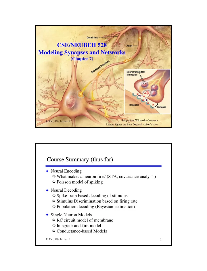
CSE/NEUBEH 528 Modeling Synapses and Networks (Chapter 7) Image from Wikimedia Commons R. Rao, 528: Lecture 8 1 Lecture figures are from Dayan & Abbott’s book Course Summary (thus far) F Neural Encoding What makes a neuron fire? (STA, covariance analysis) Poisson model of spiking F Neural Decoding Spike-train based decoding of stimulus Stimulus Discrimination based on firing rate Population decoding (Bayesian estimation) F Single Neuron Models RC circuit model of membrane Integrate-and-fire model Conductance-based Models R. Rao, 528: Lecture 8 2
Today’s Agenda F Computation in Networks of Neurons Modeling synaptic inputs From spiking to firing-rate based networks Feedforward Networks Multilayer Networks R. Rao, 528: Lecture 8 3 How do neurons connect to form networks? Using synapses! R. Rao, 528: Lecture 8 4 Image Source: Wikimedia Commons
Synapses on an actual neuron R. Rao, 528: Lecture 8 5 Image Credit: Kennedy lab, Caltech. http://www.its.caltech.edu/~mbkla What do synapses do? Spike Increase or decrease postsynaptic membrane potential R. Rao, 528: Lecture 8 6 Image Source: Wikimedia Commons
An Excitatory Synapse Input spike Spike Neurotransmitter release (e.g., Glutamate) Binds to ion channel receptors Ion channels open Na+ influx Depolarization due to EPSP (excitatory postsynaptic potential) R. Rao, 528: Lecture 8 7 Image Source: Wikimedia Commons An Inhibitory Synapse Input spike Spike Neurotransmitter release (e.g., GABA) Binds to ion channel receptors Ion channels open Cl- influx Hyperpolarization due to IPSP (inhibitory postsynaptic potential) R. Rao, 528: Lecture 8 8 Image Source: Wikimedia Commons
We want a computational model of the effects of a synapse on the membrane potential V Synapse V How do we do this? R. Rao, 528: Lecture 8 9 Flashback Membrane Model V dV ( V E ) I L e c , or equivalently: m = r m c m = R m C m m dt r A m is the membrane dV time constant ( V E ) I R m L e m dt R. Rao, 528: Lecture 8 10 Image Source: Dayan & Abbott textbook
How do we model the effects of a synapse on the membrane potential V ? ? Synapse R. Rao, 528: Lecture 8 11 Hint! Hodgkin-Huxley Model K Na dV i r I R m m m e m dt 4 3 i ( 1 / r )( V E ) g n ( V E ) g m h ( V E ) m m L K , max K Na , max Na E L = -54 mV, E K = -77 mV, E Na = +50 mV R. Rao, 528: Lecture 8 12 Image Source: Dayan & Abbott textbook
Modeling Synaptic Inputs Synaptic V conductance Synapse dV ( ) ( ) V E r g V E I R m L m s s e m dt g g P P Probability of postsynaptic channel opening s s , max rel s (= fraction of channels opened) Probability of transmitter release given an input spike R. Rao, 528: Lecture 8 13 Basic Synapse Model F Assume P rel = 1 fraction of F Model the effect of a single spike input on P s channels opened F Kinetic Model of postsynaptic channels: s Open Closed s dP s ( 1 P ) P s s s s dt Opening rate Closing rate Fraction of channels open Fraction of channels closed R. Rao, 528: Lecture 8 14
What does P s look like over time given a spike? t K ( t ) e s Exponential function K ( t ) gives reasonable fit for some synapses Others can be fit using “Alpha” function: t P max K ( t ) t e peak t R. Rao, 528: Lecture 8 15 0 peak Linear Filter Model of a Synapse Synapse Input Spike b Train b (t) b ( t ) = i δ ( t-t i ) ( t i are the input spike times , δ = delta function) Filter for K ( t ) synapse b = Synaptic conductance at b : g ( t ) g K ( t t ) b b , max i t t i t g K ( t ) ( ) d b , max b R. Rao, 528: Lecture 8 16
Example: Network of Integrate-and-Fire Neurons Excitatory synapses ( E b = 0 mV) Inhibitory synapses ( E b = -80 mV) Synchrony! dV ( ) ( )( ) V E r g t V E I R Each neuron: m L m b b e m dt E 70 mV V 54 mV Synapses : Alpha function model L thresh 1 0 ms R. Rao, 528: Lecture 8 17 peak Modeling Networks of Neurons F Option 1: Use spiking neurons Advantages : Model computation and learning based on: Spike Timing Spike Correlations/Synchrony between neurons Disadvantages : Computationally expensive F Option 2: Use neurons with firing-rate outputs (real valued outputs) Advantages : Greater efficiency, scales well to large networks Disadvantages : Ignores spike timing issues F Question: How are these two approaches related? R. Rao, 528: Lecture 8 18
Recall: Linear Filter Model of a Synapse Synapse b Input Spike Train b (t) b ( t ) = i δ ( t-t i ) ( t i are the input spike times , δ = delta function) Filter for K ( t ) synapse b = Synaptic conductance at b : g ( t ) g K ( t t ) b b , max i t t i t g K ( t ) ( ) d b , max b R. Rao, 528: Lecture 8 19 From a Single Synapse to Multiple Synapses w 1 Synaptic weights w N Spike trains 1 (t) N (t) N ( ) ( ) I t I t Total synaptic current s b b 1 t N I ( t ) w K ( t ) ( ) d s b b b 1 R. Rao, 528: Lecture 8 20
From Spiking to Firing Rate Model w 1 Synaptic weights w N Spike trains 1 (t) N (t) u N (t) Firing rate u 1 (t) t N Total Spike train b (t) I ( t ) w K ( t ) ( ) d s b b synaptic b 1 current t N Firing rate u b (t) w K ( t ) u ( ) d b b 1 b R. Rao, 528: Lecture 8 21 Simplifying the Input Current Equation w 1 Synaptic weights w N Weight vector w u N (t) Firing rate u 1 (t) Input vector u t 1 K ( t ) e Suppose synaptic filter K is exponential: s s t Differentiating w.r.t. time t , I ( t ) w K ( t ) u ( ) d s b b b dI s I w u we get s s b b dt b w I u s R. Rao, 528: Lecture 8 22
General Firing-Rate-Based Network Model F is the “activation function” Output firing rate dv v F ( I ( t )) changes like this: r s dt What happens when: Input current dI w ? changes like this: s I u s r s s dt ? r s Static input? R. Rao, 528: Lecture 8 23 Next Class: Networks F To Do: Homework 3 Finalize a final project topic and partner(s) Email Raj, Adrienne and Rich your topic and partners, or ask to be assigned to a team R. Rao, 528: Lecture 8 24
Recommend
More recommend
Explore More Topics
Stay informed with curated content and fresh updates.


![Interactive Proofs Lecture 19 And Beyond 1 So far 2 So far IP = PSPACE = AM[poly] 2 So far](https://c.sambuz.com/1028644/interactive-proofs-s.webp)
