Course Business Two new datasets on CourseWeb: vocab.csv and bpd.csv - PowerPoint PPT Presentation

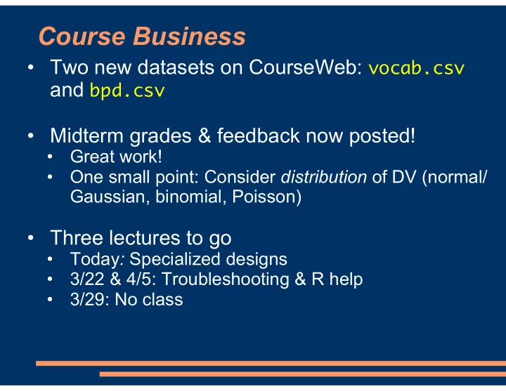
Course Business • Two new datasets on CourseWeb: vocab.csv and bpd.csv • Midterm grades & feedback now posted! • Great work! • One small point: Consider distribution of DV (normal/ Gaussian, binomial, Poisson) • Three lectures to go • Today : Specialized designs • 3/22 & 4/5: Troubleshooting & R help • 3/29: No class

Course Business • Last two weeks of the course will be final project presentations • For each, 10 min. + 5 min. for questions • Sign up on CourseWeb for your preferred day (Apr. 12 th or 19 th ) • Assignments � Final Project Presentation • Submit a response that is just your preferred date • I will assign them first come, first serve • Assignment will be returned to you on CourseWeb after the presentation with your grade from the presentation • Can also view the rubric for how the presentations will be scored • Final paper rubric also now available (due 19 th )

Week 11: Advanced Designs � Distributed Practice � Longitudinal Data � Overview � Growth Curve Analysis � Main Effect � Random Slopes � Other Variables � Quadratic & Higher Degrees � Signal Detection Theory � Why Do We Need SDT? � Sensitivity vs. Response Bias � Implementation � SDT & Other Independent Variables � Logit vs. Probit

Distributed Practice � Elika is running an experiment in which subjects envision themselves in a number of hypothetical dating scenarios (items) and rate their relationship satisfaction in that scenario. Elika is interested both in features of the scenarios & how those features may interact with the participants’ gender. Her initial model, with a maximal random effects structure, is: model1 <- lmer(Rating ~ 1 + 
 � SubjectGender * PhysicalIntimacy * EmotionalIntimacy + 
 (1 + PhysicalIntimacy * EmotionalIntimacy|Subject) + 
 (1 + SubjectGender|Item), data=dating) � Unfortunately, this model did not converge. What could Elika do as her next step?

Distributed Practice � Elika is running an experiment in which subjects envision themselves in a number of hypothetical dating scenarios (items) and rate their relationship satisfaction in that scenario. Elika is interested both in features of the scenarios & how those features may interact with the participants’ gender. Her initial model, with a maximal random effects structure, is: model1 <- lmer(Rating ~ 1 + 
 � SubjectGender * PhysicalIntimacy * EmotionalIntimacy + 
 (1 + PhysicalIntimacy * EmotionalIntimacy||Subject) + 
 (1 + SubjectGender||Item), data=dating) � Unfortunately, this model did not converge. What could Elika do as her next step? � Try taking out the correlation parameters by using || instead of |

Distributed Practice � Elika is running an experiment in which subjects envision themselves in a number of hypothetical dating scenarios (items) and rate their relationship satisfaction in that scenario. Elika is interested both in features of the scenarios & how those features may interact with the participants’ gender. Her initial model, with a maximal random effects structure, is: model1 <- lmer(Rating ~ 1 + 
 � SubjectGender * PhysicalIntimacy * EmotionalIntimacy + 
 (1 + PhysicalIntimacy * EmotionalIntimacy||Subject) + 
 (1|Item), data=dating) � Unfortunately, this model did not converge. What could Elika do as her next step? � Variance across items is often smaller. Try removing the slope by items And, use anova() to compare that model with only random � intercepts to verify that item slope does not contribute to model fit

Distributed Practice � Elika is running an experiment in which subjects envision themselves in a number of hypothetical dating scenarios (items) and rate their relationship satisfaction in that scenario. Elika is interested both in features of the scenarios & how those features may interact with the participants’ gender. Her initial model, with a maximal random effects structure, is: model1 <- lmer(Rating ~ 1 + 
 � SubjectGender * PhysicalIntimacy * EmotionalIntimacy + 
 (1 + PhysicalIntimacy * EmotionalIntimacy||Subject) + 
 (1|Item), data=dating) � Unfortunately, this model did not converge. What could Elika do as her next step? � Could just add more iterations (but this probably won’t be helpful)

Week 11: Advanced Designs � Distributed Practice � Longitudinal Data � Overview � Growth Curve Analysis � Main Effect � Random Slopes � Other Variables � Quadratic & Higher Degrees � Signal Detection Theory � Why Do We Need SDT? � Sensitivity vs. Response Bias � Implementation � SDT & Other Independent Variables � Logit vs. Probit

Vocabulary Size at 2 Years Old LEVEL 2 Neigh- Neigh- Sampled borhood borhood 1 2 NEIGHBORHOODS LEVEL 1 Child Child Child Child Sampled CHILDREN 1 2 3 4 • What kind of random-effects structure is this?

Vocabulary Size at 2 Years Old LEVEL 2 Neigh- Neigh- Sampled borhood borhood 1 2 NEIGHBORHOODS LEVEL 1 Child Child Child Child Sampled CHILDREN 1 2 3 4 • What kind of random-effects structure is this? • Two levels of nesting – sample neighborhoods, then sample children inside each neighborhood

vocab.csv: Vocabulary Size in 2 nd Year of Life LEVEL 2 Neigh- Neigh- Sampled borhood borhood 1 2 NEIGHBORHOODS LEVEL 1 Child Child Child Child Sampled CHILDREN 1 2 3 4 Child 1 Child 2 Child 3 Child 3 Assess- Assess- Assess- Assess- ment 1 ment 2 ment 2 ment 1 • Now imagine we observed each child several different times • e.g., every month over the course of a year

vocab.csv: Vocabulary Size in 2 nd Year of Life LEVEL 3 Neigh- Neigh- Sampled borhood borhood 1 2 NEIGHBORHOODS LEVEL 2 Child Child Child Child Sampled CHILDREN 1 2 3 4 LEVEL 1 Child 1 Child 2 Child 3 Child 3 Sampled TIME Assess- Assess- Assess- Assess- POINTS ment 1 ment 2 ment 2 ment 1 • This is just another level of nesting • Sample neighborhoods • Sample children within each neighborhood • Sample time points within each child

Week 11: Advanced Designs � Distributed Practice � Longitudinal Data � Overview � Growth Curve Analysis � Main Effect � Random Slopes � Other Variables � Quadratic & Higher Degrees � Signal Detection Theory � Why Do We Need SDT? � Sensitivity vs. Response Bias � Implementation � SDT & Other Independent Variables � Logit vs. Probit

Time as a Predictor Variable • We can add the effect of Time Time to our model • Here: Months since the study started • Nothing “special” about time as a predictor model1 <- lmer(VocabWords ~ 1 + Time + 
 • (1|Child) + (1|Neighborhood), data=vocab) 
 • We need to account for the nested random effects structure … can you add appropriate random intercepts ? • Tip #1: There are two levels of nesting here • Tip #2: Individual observations are nested within children, and children are nested with neighborhoods • Tip #3 : Include both Child and Neighborhood differences


 
 
 
 Time as a Predictor Variable • We can add the effect of Time Time to our model • Here: Months since the study started • Nothing “special” about time as a predictor model1 <- lmer(VocabWords ~ 1 + Time + 
 • (1|Child) + (1|Neighborhood), data=vocab) 
 • Gain of about ~55 words per month

Time as a Predictor Variable • Not necessary to have every time point represented • Dependent variable should be on same scale across time points for this to be meaningful • Time units don’t matter as long as they’re consistent Could be hours, days, years … •

Week 11: Advanced Designs � Distributed Practice � Longitudinal Data � Overview � Growth Curve Analysis � Main Effect � Random Slopes � Other Variables � Quadratic & Higher Degrees � Signal Detection Theory � Why Do We Need SDT? � Sensitivity vs. Response Bias � Implementation � SDT & Other Independent Variables � Logit vs. Probit

Longitudinal Data: Random Slopes LEVEL 3 Neigh- Neigh- Sampled borhood borhood 1 2 NEIGHBORHOODS LEVEL 2 Child Child Child Child Sampled CHILDREN 1 2 3 4 Growth Growth Rate 1 Rate 2 LEVEL 1 Child 1 Child 2 Child 3 Child 3 Sampled TIME Assess- Assess- Assess- Assess- POINTS ment 1 ment 2 ment 2 ment 1 • So far, we assume the same growth rate for all kids • Almost certainly not true! • At level 2, we’re sampling kids both with different starting points (intercepts) and growth rates (slopes)

Longitudinal Data: Random Slopes RANDOM INTERCEPTS MODEL WITH RANDOM SLOPES Kids vary in starting point, but all Allows rate of vocab acquisition to vary acquire vocabulary at the same rate across kids (as well as intercept) over this period

Longitudinal Data: Random Slopes LEVEL 3 Neigh- Neigh- Sampled borhood borhood 1 2 NEIGHBORHOODS LEVEL 2 Child Child Child Child Sampled CHILDREN 1 2 3 4 Growth Growth Rate 1 Rate 2 LEVEL 1 Child 1 Child 2 Child 3 Child 3 Sampled TIME Assess- Assess- Assess- Assess- POINTS ment 1 ment 2 ment 2 ment 1 • Can you update the model to allow the Time effect to be different for each Child ? • Tip 1: This involves some type of random slope… • Tip 2: We want a random slope of Time by Child