Course Business Midterm grades next week Two new datasets on - PowerPoint PPT Presentation
Course Business Midterm grades next week Two new datasets on CourseWeb: vocab.csv and relationship.csv Also, packages to download: languageR and lattice Four lectures to go Today : Specialized designs Then:
Week 10: Longitudinal Designs l Overview l Growth Curve Analysis l Main Effect l Random Slopes l Other Variables l Quadratic & Higher Degrees l Autocorrelation l Testing for Autocorrelation l Visualizing Autocorrelation l Direction & Lag l Why Does Autocorrelation Matter? l Cross-Lagged Models l Cross-Lagged Models l Establishing Causality
Longitudinal Data: Random Slopes LEVEL 3 Neigh- Neigh- Sampled borhood borhood 1 2 NEIGHBORHOODS LEVEL 2 Child Child Child Child Sampled CHILDREN 1 2 3 4 Growth Growth Rate 1 Rate 2 LEVEL 1 Child 1 Child 2 Child 3 Child 3 Sampled TIME Assess- Assess- Assess- Assess- POINTS ment 1 ment 2 ment 2 ment 1 • So far, we assume the same growth rate for all kids • Almost certainly not true! • At level 2, we’re sampling kids both with different starting points (intercepts) and growth rates (slopes)
Longitudinal Data: Random Slopes RANDOM INTERCEPTS MODEL WITH RANDOM SLOPES Kids vary in starting point, but all Allows rate of vocab acquisition to vary acquire vocabulary at the same rate across kids (as well as intercept) over this period
Longitudinal Data: Random Slopes LEVEL 3 Neigh- Neigh- Sampled borhood borhood 1 2 NEIGHBORHOODS LEVEL 2 Child Child Child Child Sampled CHILDREN 1 2 3 4 Growth Growth Rate 1 Rate 2 LEVEL 1 Child 1 Child 2 Child 3 Child 3 Sampled TIME Assess- Assess- Assess- Assess- POINTS ment 1 ment 2 ment 2 ment 1 • Can you update the model to allow the Time effect to be different for each Child ? • Tip 1: This involves some type of random slope… • Tip 2: We want a random slope of Time by Child
Longitudinal Data: Random Slopes model.Slope <- lmer(VocabWords ~ 1 + Time + • (1+Time|Child) + (1|Neighborhood), data=vocab) In fact, LOTS of variability in the Time slope SD is 20 words! Mean slope is 53 words/mo, but some kids might have a slope of 73 or 33
Longitudinal Data: Random Slopes • Would also be possible to have a random slope of Time by Neighborhood • If there’s clustering of growth rates at the neighborhood level model.TwoSlopes <- lmer(VocabWords ~ 1 + Time • + (1+Time|Child) + (1+Time|Neighborhood), data=vocab) • Is this are any evidence for this clustering? anova(model.Slope, model.TwoSlopes) • χ 2(2) = 0.61 p = .74 n.s.
Week 10: Longitudinal Designs l Overview l Growth Curve Analysis l Main Effect l Random Slopes l Other Variables l Quadratic & Higher Degrees l Autocorrelation l Testing for Autocorrelation l Visualizing Autocorrelation l Direction & Lag l Why Does Autocorrelation Matter? l Cross-Lagged Models l Cross-Lagged Models l Establishing Causality
Other Variables • We may want to include other variables in a longitudinal model: • Do parents frequently read picture books to the child? Time + Reading • • Effect of Reading invariant across time • Can only affect the intercept (parallel lines) Time * Reading • • Effect of Reading varies with time • Can affect intercept & slope
Other Variables: Results • Fixed-effect results with the interaction: Parental reading doesn’t affect vocab at time 0 But, results in faster vocab Growth rate for “No” group: growth 50.040 words / month (amplifies + Time effect) Growth rate for “Yes” group: 50.040 + 6.703 = 56.743 words / month e.g., Huttenlocher et al., 1991
Other Variables • Can be either: • Time-Invariant Predictor: LEVEL 3 Neigh- Same across all time points Sampled borhood 1 NEIGHBORHOODS within a subject • e.g., race/ethnicity • Level 2 or Level 3 variables LEVEL 2 Child Child Sampled CHILDREN 1 2 • Time-Varying Predictor: Varies even within a subject, from one time point to another LEVEL 1 • e.g., hours of sleep Child 1 Child 2 Sampled TIME • Level-1 variable Assess- Assess- POINTS ment 1 ment 2 • Since R automatically figures out what’s a level-1 vs. level-2 variable, we don’t have to do anything special for either kind of variable
Week 10: Longitudinal Designs l Overview l Growth Curve Analysis l Main Effect l Random Slopes l Other Variables l Quadratic & Higher Degrees l Autocorrelation l Testing for Autocorrelation l Visualizing Autocorrelation l Direction & Lag l Why Does Autocorrelation Matter? l Cross-Lagged Models l Cross-Lagged Models l Establishing Causality
Quadratic & Higher Degrees • We’ve been assuming a linear effect of time • But, it looks like vocab growth may accelerate • Growth between +2 mo. and +4 mo. is much smaller than growth between +6 mo. and +8 mo. • Suggests a curve / quadratic equation
Quadratic & Higher Degrees • Add quadratic effect (Time 2 ): model.poly <- lmer(VocabWords ~ 1 + • poly(Time,degree=2,raw=TRUE) + (1 + poly(Time,degree=2,raw=TRUE)|Child) + (1|Neighborhood), data=vocab) • degree=2 because we want Time 2 • raw=TRUE to keep the original scale of the variables (time measured in months) poly() automatically adds lower-order terms • as well • i.e., the linear term (Time)
Quadratic & Higher Degrees • Results: Intercept Linear term Quadratic term • Implied equation (approximate): • VocabWords = 40 + 11*Time + 7*Time 2 • What are predicted values if… • Time=0? • Time=1? • Time=2?
Quadratic & Higher Degrees • Results: Intercept Linear term Quadratic term • Implied equation (approximate): • VocabWords = 40 + 11*Time + 7*Time 2 • What are predicted values if… VocabWords=40+(11*0)+(7*0 2 ) = 40 • Time=0? VocabWords=40+(11*1)+(7*1 2 ) = 58 • Time=1? • Time=2? VocabWords=40+(11*2)+(7*2 2 ) = 90 • Vocab growth is accelerating (larger change from time 1 to time 2 than from time 0 to time 1)
POSITIVE QUADRATIC TREND & NO LINEAR TREND NEGATIVE QUADRATIC TREND & NO LINEAR TREND Different patterns of quadratic & linear effects describe different curves POSITIVE QUADRATIC TREND & POSITIVE LINEAR TREND NEGATIVE QUADRATIC TREND & POSITIVE LINEAR TREND
Quadratic & Higher Degrees • The Yerkes-Dodson law (Yerkes & Dodson, 1908) describes the optimal level of physiological arousal to perform a task: Low arousal results in poor performance because you are not alert enough, medium arousal results in strong performance, and high arousal results in poor performance because you are too anxious. Linear trend: Quadratic trend:
Quadratic & Higher Degrees • The Yerkes-Dodson law (Yerkes & Dodson, 1908) describes the optimal level of physiological arousal to perform a task: Low arousal results in poor performance because you are not alert enough, medium arousal results in strong performance, and high arousal results in poor performance because you are too anxious. Linear trend: NONE Quadratic trend: NEGATIVE
Quadratic & Higher Degrees • In adulthood, working memory declines the older you get (Park et al., 2002). Linear trend: Quadratic trend:
Quadratic & Higher Degrees • In adulthood, working memory declines the older you get (Park et al., 2002). Linear trend: NEGATIVE Quadratic trend: NONE
Quadratic & Higher Degrees • Aphasia is a neuropsychological disorder that disrupts speech, often resulting from a stroke. After initially acquiring aphasia, patients often experience rapid recovery in much of their language performance (dependent variable) as time (independent variable) increases. But, this recovery eventually slows down, and language performance doesn’t get much better no matter how much more time increases (e.g., Demeurisse et al., 1980). Linear trend: Quadratic trend:
Quadratic & Higher Degrees • Aphasia is a neuropsychological disorder that disrupts speech, often resulting from a stroke. After initially acquiring aphasia, patients often experience rapid recovery in much of their language performance (dependent variable) as time (independent variable) increases. But, this recovery eventually slows down, and language performance doesn’t get much better no matter how much more time increases (e.g., Demeurisse et al., 1980). POSITIVE Linear trend: NEGATIVE Quadratic trend:
Quadratic & Higher Degrees • Studies of practice and expertise (e.g., Logan, 1988) show that people learning to do a task—such as arithmetic—initially show a quick decrease in response time (dependent variable) as the amount of practice increases. However, eventually they hit the point where the task can’t possibly be done any faster, and response time reaches an asymptote and stops decreasing. Linear trend: Quadratic trend:
Quadratic & Higher Degrees • Studies of practice and expertise (e.g., Logan, 1988) show that people learning to do a task—such as arithmetic—initially show a quick decrease in response time (dependent variable) as the amount of practice increases. However, eventually they hit the point where the task can’t possibly be done any faster, and response time reaches an asymptote and stops decreasing. Linear trend: NEGATIVE POSITIVE Quadratic trend:
Quadratic & Higher Degrees • Could go up to even higher degrees (Time 3 , Time 4 …) degree=3 if highest exponent is 3 • • Degree minus 1 = Number of bends in the curve x^1 x^2 x^3 2 bends 0 bends 1 bend 0 20 40 60 80 100 0 20 40 60 80 100 -100 -50 0 50 100
Quadratic & Higher Degrees • Maximum degree of polynomial: # of time points minus 1 • Example: 2 time points perfectly fit by a line (degree 1). Nothing left for a quadratic term to explain. • But, don’t want to overfit • Probably not the case that the real underlying (population) trajectory has 6 bends in it • What degree should we include? • Theoretical considerations • If comparing conditions, look at mean trajectory across conditions (Mirman et al., 2008)
Week 10: Longitudinal Designs l Overview l Growth Curve Analysis l Main Effect l Random Slopes l Other Variables l Quadratic & Higher Degrees l Autocorrelation l Testing for Autocorrelation l Visualizing Autocorrelation l Direction & Lag l Why Does Autocorrelation Matter? l Cross-Lagged Models l Cross-Lagged Models l Establishing Causality
Longitudinal Designs • Two big questions mixed-effects models can help us answer about longitudinal data: 1) What is the overall trajectory of change across time? 2) How does an observation at one time point relate to the next time point?
Autocorrelation • So far, we’ve looked at general trajectory across time • e.g., kids who are 24 months old have larger vocabs than kids who are 18 months old • But, there may be relations among specific observations • Does reading to your kids a lot one month increase their vocab growth the next month? • Does being in a positive mood one day carry over to the next day? • Does purchasing a particular brand once make you more likely to purchase it again?
relationship.csv • One member of a dating couple rates their warmth towards the partner • For each of 10 consecutive days • First, let’s see if WarmthToday consistently increases or decreases across the 10 Day s of the study • Remember to account for nesting within couples model.time <- lmer(WarmthToday ~ 1 + Day + • (1|Couple), data=relationship) • Or: model.time <- lmer(WarmthToday ~ 1 + Day + (1 + • Day|Couple), data=relationship)
relationship.csv • No linear increase or decrease in warmth over the 10 days • Makes sense … this is a relatively short timescale • Check out the descriptives tapply(relationship$WarmthToday, • relationship$Day, mean)
Autocorrelation • We found no overall increase/decrease L I N E A R T R E N D 1 2 3 4 5 • Nevertheless, succeeding days might be more similar, even if there is no overall trend
Autocorrelation • We found no overall increase/decrease L I N E A R T R E N D + 2 3 4 5 • Nevertheless, succeeding days might be more similar, even if there is no overall trend • If you have warm feelings towards your partner one day, maybe warmer the next, too
Autocorrelation • We found no overall increase/decrease L I N E A R T R E N D + + 3 4 5 • Nevertheless, succeeding days might be more similar, even if there is no overall trend • If you have warm feelings towards your partner one day, maybe warmer the next, too
Autocorrelation • We found no overall increase/decrease L I N E A R T R E N D + + 3 - 5 • Nevertheless, succeeding days might be more similar, even if there is no overall trend • If you have warm feelings towards your partner one day, maybe warmer the next, too • If you have negative feelings, maybe less warm the next day
Autocorrelation • We found no overall increase/decrease L I N E A R T R E N D + + 3 - - • Nevertheless, succeeding days might be more similar, even if there is no overall trend • If you have warm feelings towards your partner one day, maybe warmer the next, too • If you have negative feelings, maybe less warm the next day
Autocorrelation • We found no overall increase/decrease + + 3 - - • Nevertheless, succeeding days might be more similar, even if there is no overall trend • If you have warm feelings towards your partner one day, maybe warmer the next, too • If you have negative feelings, maybe less warm the next day
Autocorrelation head(relationship, n=10) • Couple 01
Autocorrelation • These are examples of autocorrelation Couple 01 Couple 02
Autocorrelation "Maybe in order to understand mankind, we have to look at that word itself: MANKIND. Basically, it's made up of two separate words, 'mank' and 'ind.' What do these words mean? It's a mystery, and that's why so is mankind.” -- Jack Handey
Autocorrelation To understand autocorrelation , we have to look at the two separate words that make it up auto (self) + correlation • Autocorrelation refers to a variable correlating with itself, over time • Examples: • Positive mood in the morning à Positive mood in the afternoon • RT on the previous trial à RT on this trial due to waxing & waning of attention
Autocorrelation • These are examples of autocorrelation Couple 01 Couple 02
Week 10: Longitudinal Designs l Overview l Growth Curve Analysis l Main Effect l Random Slopes l Other Variables l Quadratic & Higher Degrees l Autocorrelation l Testing for Autocorrelation l Visualizing Autocorrelation l Direction & Lag l Why Does Autocorrelation Matter? l Cross-Lagged Models l Cross-Lagged Models l Establishing Causality
Testing for Autocorrelation • Is there autocorrelation in relationship warmth? • We want to test whether yesterday’s warmth predicts today’s warmth • So, we need to add WarmthYesterday as a variable • With package languageR … relationship$WarmthYesterday <- • lags.fnc(relationship, Dataframe name time='Day', Variable that identifies the time point depvar='WarmthToday', Dependent variable group='Couple’, Variable with the level-2 grouping lag= 1 ) factor (e.g., subjects or schools) • For each observation, get the value of WarmthToday from 1 day previous and store in WarmthYesterday Baayen & Milin, 2010
Testing for Autocorrelation • Is there autocorrelation in relationship warmth? • We want to test whether yesterday’s warmth predicts today’s warmth • So, we need to add WarmthYesterday as a variable head(relationship, n=13) • Day 1 for each couple gets the couple’s mean Baayen & Milin, 2010
Testing for Autocorrelation • Is there autocorrelation in relationship warmth? • Now, include WarmthYesterday in our model model.auto <- lmer(WarmthToday ~ • 1 + Day + WarmthYesterday + (1 + Day + WarmthYesterday|Couple), data=relationship)
Testing for Autocorrelation • Non-significant linear effect: No consistent increase/decrease in warmth over these 10 days X L I N E A R T R E N D 1 2 3 4 5 • But, significant autocorrelation: Adjacent days are more similar in warmth towards partner • Random walk
Autocorrelation • These are examples of autocorrelation Couple 01 Couple 02
Week 10: Longitudinal Designs l Overview l Growth Curve Analysis l Main Effect l Random Slopes l Other Variables l Quadratic & Higher Degrees l Autocorrelation l Testing for Autocorrelation l Visualizing Autocorrelation l Direction & Lag l Why Does Autocorrelation Matter? l Cross-Lagged Models l Cross-Lagged Models l Establishing Causality
Visualization of Autocorrelation • Visualization of the autocorrelation • With packages languageR and lattice : acf.fnc(xxx , • Dataframe name time='xxx ', Variable that identifies the time point x=' ', Dependent variable group=' ') Variable with the level-2 grouping factor (e.g., subjects or schools) Baayen & Milin, 2010
Visualization of Autocorrelation • Visualization of the autocorrelation • With packages languageR and lattice : acf.fnc(relationship, • Dataframe name time='Day', Variable that identifies the time point x='WarmthToday', Dependent variable group='Couple') Variable with the level-2 grouping factor (e.g., subjects or schools) Baayen & Milin, 2010
0 2 4 6 8 0 2 4 6 8 Couple36 Couple37 Couple38 Couple39 Couple40 Height of the second One box 1.0 line indicates strength of per 0.5 autocorrelation for that couple 0.0 couple -0.5 Couple29 Couple30 Couple31 Couple32 Couple33 Couple34 Couple35 1.0 0.5 0.0 -0.5 Couple22 Couple23 Couple24 Couple25 Couple26 Couple27 Couple28 1.0 0.5 0.0 -0.5 Acf Couple15 Couple16 Couple17 Couple18 Couple19 Couple20 Couple21 1.0 0.5 0.0 -0.5 Couple08 Couple09 Couple10 Couple11 Couple12 Couple13 Couple14 1.0 0.5 0.0 -0.5 Couple01 Couple02 Couple03 Couple04 Couple05 Couple06 Couple07 1.0 0.5 0.0 -0.5 0 2 4 6 8 0 2 4 6 8 0 2 4 6 8 0 2 4 6 8 Lag
Week 10: Longitudinal Designs l Overview l Growth Curve Analysis l Main Effect l Random Slopes l Other Variables l Quadratic & Higher Degrees l Autocorrelation l Testing for Autocorrelation l Visualizing Autocorrelation l Direction & Lag l Why Does Autocorrelation Matter? l Cross-Lagged Models l Cross-Lagged Models l Establishing Causality
Direction of Autocorrelation • Positive autocorrelation—Having more of something at time t means you have more of it at time t +1 • More warmth on day 3 à More warmth on day 4 • Longer RT on one trial à Longer RT on the next trial • Negative autocorrelation—Having more at time t means you have less at t +1 • e.g., homeostatic processes • Very hungry at time t à Get something to eat à Not hungry at time t +1 • Stock prices: Price increases à People sell the stock à Price decreases • Both analyzed the same way—just look at the sign to understand the effect
0 2 4 6 8 0 2 4 6 8 Positive autocorrelation. Couple36 Couple37 Couple38 Couple39 Couple40 This bar would be < 0 if 1.0 it were a negative 0.5 autocorrelation. 0.0 -0.5 Couple29 Couple30 Couple31 Couple32 Couple33 Couple34 Couple35 1.0 0.5 0.0 -0.5 Couple22 Couple23 Couple24 Couple25 Couple26 Couple27 Couple28 1.0 0.5 0.0 -0.5 Acf Couple15 Couple16 Couple17 Couple18 Couple19 Couple20 Couple21 1.0 0.5 0.0 -0.5 Couple08 Couple09 Couple10 Couple11 Couple12 Couple13 Couple14 1.0 0.5 0.0 -0.5 Couple01 Couple02 Couple03 Couple04 Couple05 Couple06 Couple07 1.0 0.5 0.0 -0.5 0 2 4 6 8 0 2 4 6 8 0 2 4 6 8 0 2 4 6 8 Lag
Autocorrelation: Lag Autocorrelation: Lag • Autocorrelation can happen at different time • Autocorrelation can happen at different time scales or lags scales or lags • Most common is lag 1: an observation correlates • Most common is lag 1: an observation correlates with the next one with the next one 1 2 3 4 1 2 3 4 5 5
Autocorrelation: Lag • Autocorrelation can happen at different time scales or lags • Most common is lag 1: an observation correlates with the next one • Lag 2: an observation correlates not with the next observation, but the one two time points later • Like the (false) idea that twins “skip a generation” • Effects that recur, but not immediately (e.g., earthquakes) 1 2 3 4 5
Autocorrelation: Lag • Autocorrelation can happen at different time scales or lags • Most common is lag 1: an observation correlates with the next one • Lag 2: an observation correlates not with the next observation, but the one two time points later • Like the (false) idea that twins “skip a generation” • Lag 3, Lag 4, etc… • Mood might have a lag 7 autocorrelation – weekly change (sad Monday, happy Friday) • But, be careful with autocorrelations >1—is there a theoretically plausible reason to expect them?
Leftmost line is lag 0— i.e., the correlation of an observation with itself This will always be 1 It’s shown for Lag 1 autocorrelation purposes of Lag 2 autocorrelation comparison Lag 3 autocorrelation
0 2 4 6 8 0 2 4 6 8 Couple36 Couple37 Couple38 Couple39 Couple40 1.0 0.5 0.0 -0.5 Couple29 Couple30 Couple31 Couple32 Couple33 Couple34 Couple35 1.0 0.5 0.0 -0.5 Couple22 Couple23 Couple24 Couple25 Couple26 Couple27 Couple28 1.0 0.5 0.0 -0.5 Acf Couple15 Couple16 Couple17 Couple18 Couple19 Couple20 Couple21 1.0 0.5 0.0 -0.5 Couple08 Couple09 Couple10 Couple11 Couple12 Couple13 Couple14 1.0 0.5 0.0 -0.5 Couple01 Couple02 Couple03 Couple04 Couple05 Couple06 Couple07 1.0 0.5 0.0 -0.5 0 2 4 6 8 0 2 4 6 8 0 2 4 6 8 0 2 4 6 8 Lag
Testing Autocorrelation, continued • Does our lag 1 autocorrelation account for the sequential dependency? • Examine the autocorrelation of the model residuals relationship$resid <- resid(model.auto) • • Now run acf.fnc() on resid rather than WarmthToday Baayen & Milin, 2010
0 2 4 6 8 0 2 4 6 8 No consistent Couple36 Couple37 Couple38 Couple39 Couple40 1.0 autocorrelation 0.5 remaining in the 0.0 data -0.5 Couple29 Couple30 Couple31 Couple32 Couple33 Couple34 Couple35 1.0 0.5 0.0 -0.5 Couple22 Couple23 Couple24 Couple25 Couple26 Couple27 Couple28 1.0 0.5 0.0 -0.5 Acf Couple15 Couple16 Couple17 Couple18 Couple19 Couple20 Couple21 1.0 0.5 0.0 -0.5 Couple08 Couple09 Couple10 Couple11 Couple12 Couple13 Couple14 1.0 0.5 0.0 -0.5 Couple01 Couple02 Couple03 Couple04 Couple05 Couple06 Couple07 1.0 0.5 0.0 -0.5 0 2 4 6 8 0 2 4 6 8 0 2 4 6 8 0 2 4 6 8 Lag
Week 10: Longitudinal Designs l Overview l Growth Curve Analysis l Main Effect l Random Slopes l Other Variables l Quadratic & Higher Degrees l Autocorrelation l Testing for Autocorrelation l Visualizing Autocorrelation l Direction & Lag l Why Does Autocorrelation Matter? l Cross-Lagged Models l Cross-Lagged Models l Establishing Causality
Why Does Autocorrelation Matter? • Autocorrelation can be an interesting research question in its own right • Important for model assumptions • A simple growth-curve model: = + + + Y i(j) γ 00 U 0j γ 10 x 1( j ) E i ( j) Time Warmth Overall Error term— Random baseline independent, intercept for identically couple • Assumes that time matters only insofar distributed as there’s a general increase/decrease with time • Otherwise, all observations from a couple equally similar or dissimilar … error terms independent
Why Does Autocorrelation Matter? • Autocorrelation can be an interesting research question in its own right • Important for model assumptions • Assumption all observations from a couple equally similar or dissimilar … error terms independent • Not true if there’s autocorrelation … observations similar in time dependent on one another • Underestimates L I N E A R T R E N D standard error à inflates Type I 1 2 3 4 5 error
Week 10: Longitudinal Designs l Overview l Growth Curve Analysis l Main Effect l Random Slopes l Other Variables l Quadratic & Higher Degrees l Autocorrelation l Testing for Autocorrelation l Visualizing Autocorrelation l Direction & Lag l Why Does Autocorrelation Matter? l Cross-Lagged Models l Cross-Lagged Models l Establishing Causality
Cross-Lagged Models • Our diary study also includes records of support attempts from the partner • Do these cause increased warmth towards the partner?
Cross-Lagged Models • Our diary study also includes records of support attempts from the partner • Do these cause increased warmth towards the partner? Wait just a darn minute! Correlation does not imply causation! You didn’t experimentally manipulate these support attempts, so you don’t know which caused which! I’VE FINALLY GOT YOU, FRAUNDORF!!
Cross-Lagged Models • Problem: Relation between support attempts & warmth is ambiguous • Support attempts could increase warmth towards partner • Warmth towards partner could motivate support attempts • A third variable could explain both TIME t Perceived warmth Relationship commitment ? Support attempt
Cross-Lagged Models • Problem: Relation between support attempts & warmth is ambiguous • But: Causes precede effects in time • Support attempt on a previous day should influence warmth now TIME t-1 TIME t Perceived warmth Support Support attempt attempt Duckworth, Tsukayama, & May, 2010
Cross-Lagged Models • Use lags.fnc() to create a SupportYesterday variable relationship$SupportYesterday <- lags.fnc(relationship, • time='Day', group='Couple', depvar='PartnerSupport', lag=1) • Then, use that in a model: model.lagged <- lmer(WarmthToday ~ 1 + Day + • SupportYesterday + (1|Couple), data=relationship) TIME t-1 TIME t Perceived warmth Support Support attempt attempt Duckworth, Tsukayama, & May, 2010
Cross-Lagged Models model.lagged <- lmer(WarmthToday ~ 1 + Day + • SupportYesterday + (1|Couple), data=relationship) TIME t-1 TIME t Perceived warmth Support Support attempt attempt Duckworth, Tsukayama, & May, 2010
Cross-Lagged Models • Warmth at t can’t be the cause of support at t -1 • Helps clarify which is the cause and which is the effect TIME t-1 TIME t Perceived warmth X Support Support attempt attempt Duckworth, Tsukayama, & May, 2010
Cross-Lagged Models • Warmth at t can’t be the cause of support at t -1 • But, warmth at time t -1 could still function as a 3 rd variable • Causes support attempts at time t -1 • Leads to greater warmth at time t (autocorrelation) TIME t-1 TIME t Perceived Perceived warmth warmth X X Support Support attempt attempt Duckworth, Tsukayama, & May, 2010
Cross-Lagged Models • To rule this out, we need to include the autocorrelative effect of perceived warmth (our DV) model.lagged2 <- lmer(WarmthToday ~ 1 + Day • + SupportYesterday + WarmthYesterday + (1|Couple), data=relationship) TIME t-1 TIME t Perceived Perceived warmth warmth X Support Support attempt attempt Duckworth, Tsukayama, & May, 2010
Cross-Lagged Models model.lagged2 <- lmer(WarmthToday ~ 1 + Day • + SupportYesterday + WarmthYesterday + (1|Couple), data=relationship) TIME t-1 TIME t Perceived Perceived warmth warmth X Support Support attempt attempt Duckworth, Tsukayama, & May, 2010
Cross-Lagged Models • Now, we are seeing a time-lagged effect of support attempts over and above what can predicted by previous warmth • No way to explain this in a model where the causation only works in reverse • Strong evidence against the reverse direct of causation TIME t-1 TIME t Perceived Perceived warmth warmth X X Support Support attempt attempt Duckworth, Tsukayama, & May, 2010
Week 10: Longitudinal Designs l Overview l Growth Curve Analysis l Main Effect l Random Slopes l Other Variables l Quadratic & Higher Degrees l Autocorrelation l Testing for Autocorrelation l Visualizing Autocorrelation l Direction & Lag l Why Does Autocorrelation Matter? l Cross-Lagged Models l Cross-Lagged Models l Establishing Causality
Recommend
More recommend
Explore More Topics
Stay informed with curated content and fresh updates.
