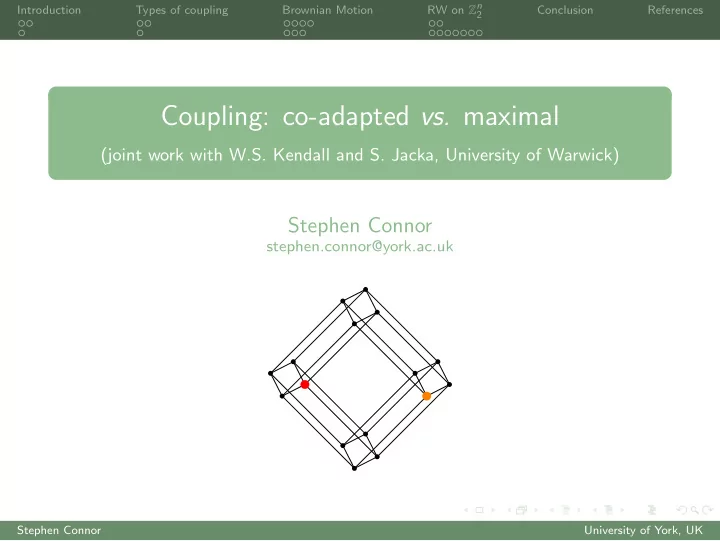
Coupling: co-adapted vs. maximal (joint work with W.S. Kendall and - PowerPoint PPT Presentation

RW on Z n Introduction Types of coupling Brownian Motion Conclusion References 2 Coupling: co-adapted vs. maximal (joint work with W.S. Kendall and S. Jacka, University of Warwick) Stephen Connor stephen.connor@york.ac.uk Stephen Connor University of York, UK

RW on Z n Introduction Types of coupling Brownian Motion Conclusion References 2 Outline Introduction 1 Coupling The coupling inequality Types of coupling 2 Maximal coupling Co-adapted coupling Brownian Motion 3 Random walk on the hypercube, Z n 4 2 Concluding remarks 5 Stephen Connor University of York, UK

RW on Z n Introduction Types of coupling Brownian Motion Conclusion References 2 Coupling Let X be a Markov process with state space S . We are interested in the situation where we have two copies of this process, X and Y , started from different states. Definition A coupling of X and Y is a process ( X ′ , Y ′ ) on S × S , such that X ′ D Y ′ D = X and = Y . That is, viewed marginally, X ′ behaves as a version of X and Y ′ as a version of Y . Stephen Connor University of York, UK

RW on Z n Introduction Types of coupling Brownian Motion Conclusion References 2 The coupling time is defined by � t : X ′ s = Y ′ � τ = inf for all s ≥ t s The coupling is successful if P ( τ < ∞ ) = 1 τ is not, in general, a stopping time (for the marginal processes nor the joint process) A ‘good’ coupling is usually one with a ‘small’ coupling time τ existence of a coupling is trivial: let X ′ and Y ′ be independent until they first meet, then stay together this idea goes back to Doeblin (1938) a major use of coupling is to provide information about the convergence of X ... Stephen Connor University of York, UK

RW on Z n Introduction Types of coupling Brownian Motion Conclusion References 2 The coupling inequality Definition Let µ and ν be probability measures defined on S . The total variation distance between µ and ν is given by � µ − ν � TV = sup ( µ ( A ) − ν ( A )) A ⊂S Stephen Connor University of York, UK

RW on Z n Introduction Types of coupling Brownian Motion Conclusion References 2 The coupling inequality Definition Let µ and ν be probability measures defined on S . The total variation distance between µ and ν is given by � µ − ν � TV = sup ( µ ( A ) − ν ( A )) A ⊂S Lemma (The coupling inequality) Let ( X , Y ) be a coupling as above. Then � P ( X t ∈ · ) − P ( Y t ∈ · ) � TV ≤ P ( τ > t ) . Stephen Connor University of York, UK

RW on Z n Introduction Types of coupling Brownian Motion Conclusion References 2 Maximal coupling It is well known that there exists a maximal coupling of X and Y (Griffeath, 1975); that is, a joint process ( X ∗ , Y ∗ ) with coupling time τ ∗ satisfying t ∈ · ) � TV = P ( τ ∗ > t ) . � P ( X ∗ t ∈ · ) − P ( Y ∗ Thus there exists a successful coupling for X if and only if X is weakly ergodic Stephen Connor University of York, UK

RW on Z n Introduction Types of coupling Brownian Motion Conclusion References 2 Although a maximal coupling is known to exist, such a coupling is typically (at best) non-Markovian, unintuitive, and very difficult to compute explicitly – they are rarely used in practical applications Stephen Connor University of York, UK

RW on Z n Introduction Types of coupling Brownian Motion Conclusion References 2 Although a maximal coupling is known to exist, such a coupling is typically (at best) non-Markovian, unintuitive, and very difficult to compute explicitly – they are rarely used in practical applications Stephen Connor University of York, UK

RW on Z n Introduction Types of coupling Brownian Motion Conclusion References 2 Although a maximal coupling is known to exist, such a coupling is typically (at best) non-Markovian, unintuitive, and very difficult to compute explicitly – they are rarely used in practical applications Stephen Connor University of York, UK

RW on Z n Introduction Types of coupling Brownian Motion Conclusion References 2 Co-adapted coupling Definition ( X , Y ) is called co-adapted if X and Y are both Markov with respect to a common filtration ( F t ). (We don’t require that ( X , Y ) is Markov w.r.t. ( F t ).) Stephen Connor University of York, UK

RW on Z n Introduction Types of coupling Brownian Motion Conclusion References 2 Co-adapted coupling Definition ( X , Y ) is called co-adapted if X and Y are both Markov with respect to a common filtration ( F t ). (We don’t require that ( X , Y ) is Markov w.r.t. ( F t ).) It now suffices to study the first collision time of X and Y → X and Y can be made to agree from this time onwards co-adapted couplings are much more intuitive (neither process is allowed to ‘cheat’ by looking into the future) maximal couplings are in general not co-adapted Stephen Connor University of York, UK

RW on Z n Introduction Types of coupling Brownian Motion Conclusion References 2 Co-adapted coupling Definition ( X , Y ) is called co-adapted if X and Y are both Markov with respect to a common filtration ( F t ). (We don’t require that ( X , Y ) is Markov w.r.t. ( F t ).) It now suffices to study the first collision time of X and Y → X and Y can be made to agree from this time onwards co-adapted couplings are much more intuitive (neither process is allowed to ‘cheat’ by looking into the future) maximal couplings are in general not co-adapted But how good can a co-adapted coupling be? Stephen Connor University of York, UK

RW on Z n Introduction Types of coupling Brownian Motion Conclusion References 2 Brownian motion: a maximal coupling Consider two Brownian motions, X and Y , on R , with X 0 = x and Y 0 = y (and x ≥ y ). Write p t ( x , u ) = e − ( u − x ) 2 / 2 t √ . 2 π t It is simple to calculate the total variation distance between these two processes at any time t using the following result... Stephen Connor University of York, UK

RW on Z n Introduction Types of coupling Brownian Motion Conclusion References 2 Lemma For probability measures µ and ν , let µ ∧ ν be their greatest common component, and let λ be a measure that dominates µ and ν . Write f = d µ f ′ = d ν d λ , d λ . Then � ( f ∧ f ′ ) d λ . � µ − ν � TV = 1 − Stephen Connor University of York, UK

RW on Z n Introduction Types of coupling Brownian Motion Conclusion References 2 y x So... � ( x + y ) / 2 �L ( X t ) − L ( Y t ) � = 1 − 2 p t ( x , z ) dz −∞ � ( x − y ) / 2 � = Erf √ 2 t � � = P x τ ( x + y ) / 2 > t . where τ ( x + y ) / 2 = inf { t ≥ 0 | X t = ( x + y ) / 2 } . Stephen Connor University of York, UK

RW on Z n Introduction Types of coupling Brownian Motion Conclusion References 2 y x So... � ( x + y ) / 2 �L ( X t ) − L ( Y t ) � = 1 − 2 p t ( x , z ) dz −∞ � ( x − y ) / 2 � = Erf √ 2 t � � = P x τ ( x + y ) / 2 > t . where τ ( x + y ) / 2 = inf { t ≥ 0 | X t = ( x + y ) / 2 } . Stephen Connor University of York, UK

RW on Z n Introduction Types of coupling Brownian Motion Conclusion References 2 y x So... � ( x + y ) / 2 �L ( X t ) − L ( Y t ) � = 1 − 2 p t ( x , z ) dz −∞ � ( x − y ) / 2 � = Erf √ 2 t � � = P x τ ( x + y ) / 2 > t . where τ ( x + y ) / 2 = inf { t ≥ 0 | X t = ( x + y ) / 2 } . Stephen Connor University of York, UK

RW on Z n Introduction Types of coupling Brownian Motion Conclusion References 2 Thanks to the symmetry of BM, this shows that reflection coupling is maximal for X and Y . In other words, if we define Y by � y − ( X t − x ) for t ≤ τ ( x + y ) / 2 Y t = X t for t > τ ( x + y ) / 2 , then � � �L ( X t ) − L ( Y t ) � = P x τ ( x + y ) / 2 > t = P ( X t � = Y t ) . x x � y 2 y Stephen Connor University of York, UK

RW on Z n Introduction Types of coupling Brownian Motion Conclusion References 2 Altering the initial conditions Note that this reflection coupling is co-adapted Stephen Connor University of York, UK

RW on Z n Introduction Types of coupling Brownian Motion Conclusion References 2 Altering the initial conditions Note that this reflection coupling is co-adapted But what if we now alter the starting conditions, so that X 0 = x is fixed, but Y 0 ∼ N(0 , σ 2 )? Stephen Connor University of York, UK

RW on Z n Introduction Types of coupling Brownian Motion Conclusion References 2 Altering the initial conditions Note that this reflection coupling is co-adapted But what if we now alter the starting conditions, so that X 0 = x is fixed, but Y 0 ∼ N(0 , σ 2 )? Perhaps surprisingly... Lemma Under these initial conditions, reflection coupling for the pair of Brownian motions ( X , Y ) is not maximal Stephen Connor University of York, UK