Couplage des quations de St-Venant 1D-2D et assimilation - PowerPoint PPT Presentation
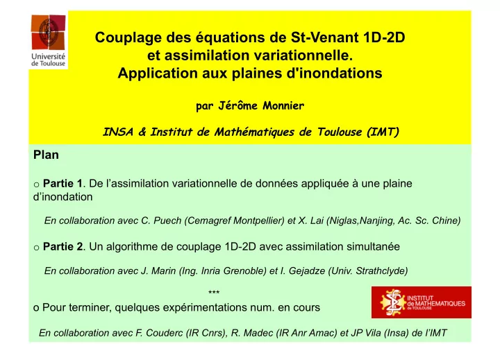
Couplage des quations de St-Venant 1D-2D et assimilation variationnelle. Application aux plaines d'inondations par Jrme Monnier INSA & Institut de Mathmatiques de Toulouse (IMT) Plan o Partie 1 . De lassimilation variationnelle
Couplage des équations de St-Venant 1D-2D et assimilation variationnelle. Application aux plaines d'inondations par Jérôme Monnier INSA & Institut de Mathématiques de Toulouse (IMT) Plan o Partie 1 . De l’assimilation variationnelle de données appliquée à une plaine d’inondation En collaboration avec C. Puech (Cemagref Montpellier) et X. Lai (Niglas,Nanjing, Ac. Sc. Chine) o Partie 2 . Un algorithme de couplage 1D-2D avec assimilation simultanée En collaboration avec J. Marin (Ing. Inria Grenoble) et I. Gejadze (Univ. Strathclyde) *** o Pour terminer, quelques expérimentations num. en cours En collaboration avec F. Couderc (IR Cnrs), R. Madec (IR Anr Amac) et JP Vila (Insa) de l’IMT
Part 1. Mosel river (at border France-Germany) . Flow configuration Upstream Flat plain (slope 0.05%) Length: 28 km Narrow valley at downstream Propagation velocity of the flood peak: 2 km/h Downstream Peak discharge: 1450 m3/s
Image analysis SAR image Step 1: Extracting waters: a fuzzy mapping… Step 2: Transforming 2D in 3D by merging image and DTM Step 3: Localization of informative points for local h values (ie. no trees, no urban, no steep slopes) downstream Step 4: “hydraulic coherence” imposed (min-max elevation following the steepest descent) Final Result: elevation h at “image blocks” with uncertainty estimates (+/- 15 cm in average) downstream Work done by C. Puech et al. Cemagref Montpellier, France Refs. [Hostache-Puech et al] Revue teledetection’06 [Raclot] Int. J. remote-sensing’06 [Puech-Raclot] Hydro. processes‘02
Summary of data available Data 1) SAR image After analysis local H-values at image time downstream with quantified uncertainties (+/-15cm) By [Puech et al.’06] Data 2) In-situ measurements Boundary conditions known: q at gauge station (EDF) q at upstream & h at downstream Plot: q at the beginning & the end of the flood event Plot: discharges at downstream & upstream
Variational Data Assimilation (4D-var) / Optimal control Adjoint method Forward model : 2D S.W.E. inviscid, in var. (h, qx, qy). Cost function. The control variable k = Manning coef. or inflow discharge + I.C. Image term: net mass flux Obs. at gauge station Local sensitivity analysis: One (1) run of the forward + adjoint models gives the gradient value hence a local sensitivity information Calibration: optimal control loop Our software DassFlow (see webpage) o Forward models: SWEs. Also: transport, sedimentation (FV), Stokes ALE non-newtonian(FE) o FV schemes: explicit HLLC or implicit Van Leer. o Adjoint code: automatic differenciation (Tapenade software, Inria) o From libraries: minimization (BFGS, Inria), linear algebra (Mumps, U. Toulouse) o MPI Fortran codes
Optimal control process DassFlow: Data Assimilation for Free-Surface Flows. Computational platform
Mosel river flood-plain flow: calibration of Manning-Strickler coefficients using 10 land-use (with main channel = constant Manning coef.) Water elevation at image bocks (in red): calibration by hand (forward run, pink) vs VDA (4D-var, blue) vertical bars = observed h from image with computed uncertainty Ref. [Hostache, Lai, Monnier, Puech] J Hydrology’10 Imposing “hydraulic coherence”,mean uncertainty bars (in red) decrease from +/-40cm to +/- 15 cm The 4D-var process (VDA) improved greatly the hydraulic model calibrated « by hand »
Sensitivity analysis Refs. [Lai, Monnier] J. Hydrology’09 without a-priori « Manning-area decomposition » [Hostache, Lai, Monnier, Puech] i.e. no land-use decomposition J. Hydrology’10 Local sensitivity analysis Result: sensitive Manning areas one needs to focus on few Manning areas inside the main channel Preliminary sensitivity analysis runs: 1) improve the understanding of the flow 2) lead to a more reliable definition of Manning-areas
Part 2. Coupling 1D-2D SWE and simultaneous assimilation Basic idea o Given a « global » flow model, superpose locally a « zoom » model on it, while keeping the existing geometry and mesh of the global model. Local zoom model: richer physics, finest grids. o In a variational data assimilation context, take advantage of the optimal control process and data in order to: Couple both models (i.e. quantify the information) Assimilate local data represented by the zoom into the global model The local zoom model can be viewed as a mapping operator. Flood plain Global model = 1D-net river branche(s). 1D SWE (St-Venant). Local model = flood plain. 2D SWE (St-Venant). Typical ratios of spatio-temporal grids 1D/2D: Dx~10 Dt~100
Global model: 1D SWE with its 2D coupling source term Classical 1D St-Venant equations S: wet cross-section in main channel ; Q: discharge If over-flowing and/or lateral filling, derivation from 3D Navier-Stokes eqns gives: If the canal width variations are small, if u is nearly constant over the cross section, if (u, v) do not depend on z on lateral boundaries, : normal discharges at lateral bdry k : tangent component of the z-mean value of u at lateral bdry k
Local model: 2D SWE (non viscous) h : water elevation ; q : 2D discharge Conservative form of 2D SWE with topography and friction source terms: 2D 1D information transfer Open-boundaries continuity of incoming characteristics at interfaces : where the 2D characteristics are: (linearized 2D SWE, no topo, no friction) associated to eigenvalues:
Numerical schemes: A-priori, grids are non-matching superposed F.V. schemes 1D-2D o Discretization for the source term in the 1D model = component #1 of the numerical flux : up-winding upon the sign of intermediate wave speed dynamical over-flowing / filling lateral flows taken into account Numerical validation. Schwarz 2Dover1D vs full 2D-model: perfect matched results o Globally well-balanced ? Since: • An 1D topography term appears in the 1D SWE, • A 2D topography term appears in the 2D SWE (thus implicitely in the 2D term of 1D SWE too), Is the resulting global FV scheme 1D-2D well-balanced ? Answer: If both 1D conservative schemes (1D&2D models) are separitively well-balanced, then the coupled global scheme 1D-2D is well-balanced too. Part done with E. Fernandez-Nieto, univ. Sevilla, Spain o Ex. of explicit F.V. schemes possible: HLL / HLLC, Roe, Russanov Ref [Fernandez-Marin-Monnier] ’10
Algorithm of coupling: two approaches compared We seek to superpose the 2D model (local zoom) over the 1D global model: 2D SWE with fine grids over 1D SWE with coarse grids 1) Schwarz type algorithms With a Domain Decomposition (D.D.) approach: for SWE 1D-2D-1D see eg. [Miglio-Perroto-Saleri’05] With a Superposition approach: for SWE 1D-2D-1D, see the following num. tests, [Gejadze-Monnier’07] [Fernandez-Marin-Monnier]’10 2) A minimization / optimal control approach the present Joint Assimilation Coupling (JAC) algorithm(s) we assume to be in a context of variational data assimilation, we take advantage of the existing optimal control process and data… *** Principle of JAC algo. A «relaxed» coupled problem (one way coupled model) is controlled: Control of the quantities (characteristics) at interfaces, Minimization of Delta(quantities) at interfaces. o Some references related to the subject - Virtual-control method : optimal control of conditions at interfaces/link with D.D. See [Lions-Pironneau]’98 & ‘99, [Lions’00] Heterogeneous coupling by virtual control, see [Gervasio-Lions-Quarteroni’01]etc - Augmented lagrangian approach : see e.g. [LeTallec-Sassi]’96 - Nested multi-d river models with a-posteriori selection criteria see [Amara-Capatina-Trujillo]’04 + Petrau PhD’09
Refs Our coupling algorithm: Joint Assimilation–Coupling (JAC) [Marin, Monnier] ’09 [Gejadze, Monnier] ‘07 Principle: 1) One-way coupling term is relaxed (incoming charac. at interfaces), It is added into the cost function (extra term) 2) Data are used to quantify the coupling information Augmented cost function: with If the term vanishes after minimization process then weak continuity of incoming characteristics at interfaces is obtained An other version of JAC algorithm: the « sequential » JAC
The « relaxed » JAC algorithm Principle: We control the one way coupled model 2D 1D *** Features: • Multi-objectives optimization: Need to balance « by hand » observation terms, regul. terms & coupling terms • Convergence looks to be quite robust (academic test case) *** Augmented cost function:
Bathymetry Academic numerical test: Obs: h at station #2 Identification of Qin in the 1D-model Observations : station 2 in the flooding area only read by the « local » zoom 2D model Problem: identify the inflow discharge in the 1D « global » model Incom charac at outflow identified Inflow discharge identified Minimization process Ref. [Marin, Monnier] ’09 Incom charac at inflow identified
An other version: the « sequential » JAC algorithm Step 1 • Calibration (minimization) of the 2D zoom model only • Save the resulting source term Step 2 • Calibration (minimization) of the 1D global model *** Features • The adjoint codes are separated • the two optimization problems are solved sequentially But convergence is less robust, and a « blind period » must be removed between both steps…
A comparison JAC vs Schwarz algorithm global in time Same coupling configuration 1D-2D non-matching grids (but constant slopes) Ratio 1D/2D: space =10 , time =100
Recommend
More recommend
Explore More Topics
Stay informed with curated content and fresh updates.
