Cosmic Calibration Katrin Heitmann Statistical Challenges for - PowerPoint PPT Presentation
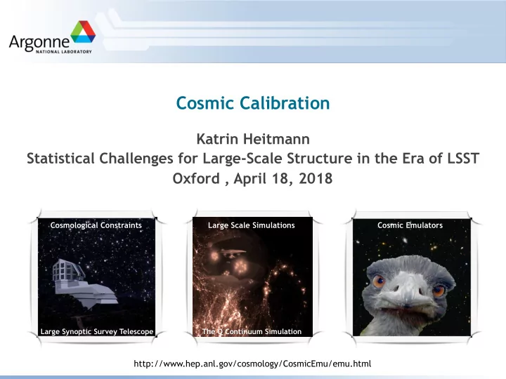
Cosmic Calibration Katrin Heitmann Statistical Challenges for Large-Scale Structure in the Era of LSST Oxford , April 18, 2018 Cosmological Constraints Large Scale Simulations Cosmic Emulation Cosmic Emulators Large Synoptic Survey Telescope
Cosmic Calibration Katrin Heitmann Statistical Challenges for Large-Scale Structure in the Era of LSST Oxford , April 18, 2018 Cosmological Constraints Large Scale Simulations Cosmic Emulation Cosmic Emulators Large Synoptic Survey Telescope The Q Continuum Simulation http://www.hep.anl.gov/cosmology/CosmicEmu/emu.html
Thanks to many collaborators! • The Beginnings -- Proof of Concept (Heitmann et al. 2006, Habib et al. 2007) • The Coyote Universe + Extension (Heitmann et al. 2009, 2010, 2013, Lawrence et al. 2010) • Emulators beyond P(k) (Kwan et al. 2013a,b) • The Mira-Titan Universe (Heitmann et al. 2015, Lawrence et al. 2017, Kwan et al., Bocquet et al in prep.) + HACC team
Thanks to many collaborators! • The Beginnings -- Proof of Concept (Heitmann et al. 2006, Habib et al. 2007) • The Coyote Universe + Extension (Heitmann et al. 2009, 2010, 2013, Lawrence et al. 2010) • Emulators beyond P(k) (Kwan et al. 2013a,b) • The Mira-Titan Universe (Heitmann et al. 2015, Lawrence et al. 2017, Kwan et al., Bocquet et al in prep.) + HACC team
Thanks to many collaborators! • The Beginnings -- Proof of Concept (Heitmann et al. 2006, Habib et al. 2007) • The Coyote Universe + Extension (Heitmann et al. 2009, 2010, 2013, Lawrence et al. 2010) • Emulators beyond P(k) (Kwan et al. 2013a,b) • The Mira-Titan Universe (Heitmann et al. 2015, Lawrence et al. 2017, Kwan et al., Bocquet et al in prep.) + HACC team
Cosmic Calibration: Solving the Inverse Problem • Challenge: To extract cosmological constraints from observations in nonlinear regime, need to run Marko Chain Monte Carlo code; input: 10,000 - 100,000 different models • Direct simulations: Cost estimate • HACC on Titan (fastest system in the US, 5th in the world) • 10 simulations fit on full machine, 24 hours per simulation • For 100,000 simulations this translates to ~30 years • Current strategy: Fitting functions for e.g. P(k), accurate at 10% level, this is not good enough! • Our alternative: Emulators, fast prediction schemes built from a manageable set of simulations • “ Ingredients”: Optimal sampling methods to decide which models to simulate, efficient representation of simulation outcome, powerful interpolation scheme • Example here: Power spectrum emulator
Cosmic Calibration Framework Design optimal simulation Modeling/Sims; Observations; • Step 1: Design simulation campaign over (~20) parameter range campaign, rule of thumb: O(10) Observations+Modeling models for each parameter • Step 2: Carry out simulation Run suite of simulations (40,100,...) with chosen campaign and extract quantity of parameter values interest, in our case, power spectrum • Step 3: Choose suitable Statistics Package (Gaussian Process interpolation scheme to Modeling, MCMC) interpolate between models, here Gaussian Processes • Step 4: Build emulator Response Calibration Observation surface; • Step 5: Use emulator to analyze Distribution input emulator data, determine model inadequacy, refine simulation and modeling strategy... Model Predictive inadequacy, Distribution self calibration Katrin Heitmann, Los Alamos National Laboratory Benasque Cosmology Workshop, August 2010
The Coyote Simulation Design for wCDM Cosmologies The (original) Coyote Universe • Observational considerations Priors: ‣ CMB provides very accurate 0.020 ≤ ω ≤ 0.025 b 0.11 ≤ ω ≤ 0.15 measurements of “vanilla m 0.85 ≤ n ≤ 1.05 parameters” s -1.3 ≤ w ≤ -0.7 ‣ In particular, ω , ω , n known b m s 0.6 ≤σ ≤ 0.9 at the 2-3% level 8 ‣ w, σ less well known 8 Design Parameters • For good emulator performance Derived Parameters from very small number of runs ‣ Not too broad priors ‣ Not too many parameters Katrin Heitmann, Los Alamos National Laboratory Benasque Cosmology Workshop, August 2010
The Coyote Universe Priors: 0.020 ≤ ω ≤ 0.025 b 0.11 ≤ ω ≤ 0.15 m 0.85 ≤ n ≤ 1.05 s -1.3 ≤ w ≤ -0.7 0.6 ≤ σ ≤ 0.9 8 • 37 model runs + Λ CDM ‣ 16 low resolution realizations (green) ‣ 4 medium resolution realizations (red) ‣ 1 high resolution realization (blue) ‣ 11 outputs per run between z = 0 - 3 • Restricted priors to minimize necessary number of runs • 1.3 Gpc boxes, m p ~10 ¹¹ M . • ~1000 simulations, 60TB ° Katrin Heitmann, Los Alamos National Laboratory Benasque Cosmology Workshop, August 2010 Background Visualization with ParaView by J. Woodring
Next step: Smooth Power Spectrum • Each simulation represents one possible realization of the Universe in a finite volume • Need smooth prediction for building the emulator for each Gadget model PM, 2048 ³ PM, 1024 ³ • Major challenge: Make sure that baryon features are not washed out or enhanced due to realization scatter Baryon wiggles • Construct smooth power spectra using a process convolution model (Higdon 2002) • Basic idea: calculate moving ∆ 2 ( k ) = k 3 P ( k ) ~ ~ k ) = h δ 2 ( average using a kernel whose 2 π 2 ; P ( k ) i width is allowed to change to account for non-stationarity Katrin Heitmann, Los Alamos National Laboratory Benasque Cosmology Workshop, August 2010
Next step: Smooth Power Spectrum • Each simulation represents one possible realization of the Universe in a finite volume • Need smooth prediction for building the emulator for each Gadget model PM, 2048 ³ PM, 1024 ³ • Major challenge: Make sure that baryon features are not washed out or enhanced due to realization scatter Baryon wiggles • Construct smooth power spectra using a process convolution model (Higdon 2002) • Basic idea: calculate moving ∆ 2 ( k ) = k 3 P ( k ) ~ ~ k ) = h δ 2 ( average using a kernel whose 2 π 2 ; P ( k ) i Coyote III, Process convolution width is allowed to change to account for non-stationarity Katrin Heitmann, Los Alamos National Laboratory Benasque Cosmology Workshop, August 2010
The Interpolation Scheme: Gaussian Processing • Cosmological Number of After simulation design parameters parameters, 5 specification: Build Number of basis interpolation scheme that functions, here: 5 p η ⇢ ∆ 2 ( k , z ) � yields predictions for any ∑ θ [ 0 , 1 ] p θ = φ i ( k , z ) w i ( θ )+ ε ln ∈ cosmology within the priors 2 π k 3 / 2 i = 1 Basis functions, Weights, here: • Model simulation outputs using here: PC basis GP model a - dimensional basis p η representation ‣ Find suitable set of orthogonal mean PC basis 1 PC basis 2 basis vectors , here: φ i ( k , z ) Principal Component Analysis ! ln P 0.1 ! ln P 0.1 0 ln P 0 0 ! 2 ‣ 0 0 0 ! 4 ! 0.1 ! 0.1 5 PC bases needed, fifth PC ! 6 ! 0.2 ! 0.2 ! 3 ! 3 ! 3 .5 .5 .5 basis pretty flat ! 2 ! 2 ! 2 ! 1 ! 1 ! 1 z z z 1 1 1 0 0 0 log k log k log k ‣ Next step: modeling the weights PC basis 3 PC basis 4 PC basis 5 ‣ Here: Gaussian Process modeling (non-parametric ! ln P 0.1 ! ln P 0.1 ! ln P 0.1 0 0 0 0 0 0 ! 0.1 ! 0.1 ! 0.1 regression approach, local ! 0.2 ! 0.2 ! 0.2 ! 3 ! 3 ! 3 .5 .5 .5 interpolator; specified by mean time ! 2 ! 2 ! 2 ! 1 ! 1 ! 1 z z z 1 1 1 0 0 0 function and covariance log k log k log k Basis functions function) Katrin Heitmann, Los Alamos National Laboratory Benasque Cosmology Workshop, August 2010
The Cosmic Emu(lator) • Prediction tool for matter power spectrum has been constructed • Accuracy within specified priors between z=0 and z=1 out to k=1 h / Mpc at the 1% level achieved • Emulator has been publicly released, C code (Lawrence et al., 2010) • Extension: Includes a additional parameter, covers smaller scales and earlier times (Heitmann et al., 2014) ‣ Nested simulations to cover large k-range ‣ Approach degrades accuracy to ~3% Emulator performance: 1% Comparison of prediction and simulation output for a model not used to build 1% emulator at 6 redshifts. Katrin Heitmann, Los Alamos National Laboratory Benasque Cosmology Workshop, August 2010
The Cosmic Emu(lator) • Prediction tool for matter power spectrum has been constructed • Accuracy within specified priors between z=0 and z=1 out to k=1 h / Mpc at the 1% level achieved • Emulator has been publicly released, C code (Lawrence et al., 2010) • Extension: Includes a additional parameter, covers smaller scales and earlier times (Heitmann et al., 2014) ‣ Nested simulations to cover large k-range ‣ Approach degrades accuracy to ~3% Emulator performance: 1% Comparison of prediction and simulation output for a model not used to build 1% emulator at 6 redshifts. Katrin Heitmann, Los Alamos National Laboratory Benasque Cosmology Workshop, August 2010
The FrankenEmu Challenge 1e+05 M019 M037 10000 1000 3 ] P(k) [Mpc 100 Shot noise limit P shot ( k ) = ( L/N p ) 3 10 1 Nyquist limit 0.1 k Ny = π N p /L 0.01 1e+05 10000 1000 3 ] P(k) [Mpc z=0 100 RPT z=0 1300 Mpc 10 z=4 365 Mpc 1 180 Mpc z=4 0.1 90 Mpc 0.01 0.001 0.01 0.1 1 10 0.001 0.01 0.1 1 10 -1 ] -1 ] k [Mpc k [Mpc Katrin Heitmann, Los Alamos National Laboratory Benasque Cosmology Workshop, August 2010
Recommend
More recommend
Explore More Topics
Stay informed with curated content and fresh updates.
