Convergence rates in convex optimization Beyond the worst-case with - PowerPoint PPT Presentation
Convergence rates in convex optimization Beyond the worst-case with the help of geometry Guillaume Garrigos with Lorenzo Rosasco and Silvia Villa cole Normale Suprieure Journes du GdR MOA/MIA - Bordeaux - 19 Oct 2017 Guillaume Garrigos
Convergence rates in convex optimization Beyond the worst-case with the help of geometry Guillaume Garrigos with Lorenzo Rosasco and Silvia Villa École Normale Supérieure Journées du GdR MOA/MIA - Bordeaux - 19 Oct 2017 Guillaume Garrigos 1/27
Introduction Setting: X Hilbert space, f : X → R ∪ { + ∞} convex l.s.c. Problem: Minimize f ( x ) , x ∈ X . Tool: My favorite algorithm. Guillaume Garrigos 2/27
Introduction Setting: X Hilbert space, f : X → R ∪ { + ∞} convex l.s.c. Problem: Minimize f ( x ) , x ∈ X . Tool: My favorite algorithm. As optimizers, we often face the same questions concerning the convergence of an algorithm: (Qualitative result) For the iterates ( x n ) n ∈ N : weak, strong convergence? (Quantitative result) For the iterates and/or the values: sublinear O ( n − α ) rates, linear O ( ε n ) , superlinear ? Guillaume Garrigos 2/27
Introduction Setting: X Hilbert space, f : X → R ∪ { + ∞} convex l.s.c. Problem: Minimize f ( x ) , x ∈ X . Tool: My favorite algorithm. As optimizers, we often face the same questions concerning the convergence of an algorithm: (Qualitative result) For the iterates ( x n ) n ∈ N : weak, strong convergence? (Quantitative result) For the iterates and/or the values: sublinear O ( n − α ) rates, linear O ( ε n ) , superlinear ? It depends on the algorithm and the assumptions made on f . Guillaume Garrigos 2/27
Introduction Setting: X Hilbert space, f : X → R ∪ { + ∞} convex l.s.c. Problem: Minimize f ( x ) , x ∈ X . Tool: My favorite algorithm. As optimizers, we often face the same questions concerning the convergence of an algorithm: (Qualitative result) For the iterates ( x n ) n ∈ N : weak, strong convergence? (Quantitative result) For the iterates and/or the values: sublinear O ( n − α ) rates, linear O ( ε n ) , superlinear ? It depends on the algorithm and the assumptions made on f . Here we will essentially consider first order descent methods, and more simply the forward-backward method. Guillaume Garrigos 2/27
Introduction Setting: X Hilbert space, f : X → R ∪ { + ∞} convex l.s.c. Problem: Minimize f ( x ) , x ∈ X . Tool: My favorite algorithm. As optimizers, we often face the same questions concerning the convergence of an algorithm: (Qualitative result) For the iterates ( x n ) n ∈ N : weak, strong convergence? (Quantitative result) For the iterates and/or the values: sublinear O ( n − α ) rates, linear O ( ε n ) , superlinear ? It depends on the algorithm and the assumptions made on f . Here we will essentially consider first order descent methods, and more simply the forward-backward method. Guillaume Garrigos 2/27
Contents Classic theory 1 Better rates with the help of geometry 2 Identifying the geometry of a function Exploiting the geometry Inverse problems in Hilbert spaces 3 Linear inverse problems Sparse inverse problems Guillaume Garrigos 3/27
Classic convergence results Let f = g + h be convex, with h L -Lipschitz smooth Let x n + 1 = prox λ g ( x n − λ ∇ h ( x n )) , λ ∈ ] 0 , 2 / L [ . Theorem (general convex case) argmin f = ∅ : x n diverges, no rates for f ( x n ) − inf f . argmin f � = ∅ : x n weakly converges to x ∞ ∈ argmin f , and � n − 1 � f ( x n ) − inf f = o . Guillaume Garrigos 4/27
Classic convergence results Let f = g + h be convex, with h L -Lipschitz smooth Let x n + 1 = prox λ g ( x n − λ ∇ h ( x n )) , λ ∈ ] 0 , 2 / L [ . Theorem (general convex case) argmin f = ∅ : x n diverges, no rates for f ( x n ) − inf f . argmin f � = ∅ : x n weakly converges to x ∞ ∈ argmin f , and � n − 1 � f ( x n ) − inf f = o . Theorem (strongly convex case) Assume that f is strongly convex. Then x n strongly converges to x ∞ ∈ argmin f , and both iterates and values converge linearly. Guillaume Garrigos 4/27
Classic convergence results Assume f to be convex and ( x n ) n ∈ N be generated by forward-backward. function values iterates argmin f = ∅ o ( 1 ) diverge o ( n − 1 ) argmin f � = ∅ weak convergence s. convex linear linear Guillaume Garrigos 5/27
Classic convergence results Assume f to be convex and ( x n ) n ∈ N be generated by forward-backward. function values iterates argmin f = ∅ o ( 1 ) diverge o ( n − 1 ) argmin f � = ∅ weak convergence ? ? ? s. convex linear linear Guillaume Garrigos 5/27
Classic convergence results Assume f to be convex and ( x n ) n ∈ N be generated by forward-backward. function values iterates argmin f = ∅ o ( 1 ) diverge o ( n − 1 ) argmin f � = ∅ weak convergence ? ? ? ? linear linear Guillaume Garrigos 5/27
Classic convergence results Assume f to be convex and ( x n ) n ∈ N be generated by forward-backward. function values iterates argmin f = ∅ o ( 1 ) diverge o ( n − 1 ) argmin f � = ∅ weak convergence ? ? ? ? linear linear − → Use geometry! Guillaume Garrigos 5/27
Known examples A ∈ L ( X , Y ) , y ∈ Y . f ( x ) = 1 2 � Ax − y � 2 , x n + 1 = x n − τ A ∗ ( Ax n − y ) If R ( A ) is closed, linear convergence. Guillaume Garrigos 6/27
Known examples A ∈ L ( X , Y ) , y ∈ Y . f ( x ) = 1 2 � Ax − y � 2 , x n + 1 = x n − τ A ∗ ( Ax n − y ) If R ( A ) is closed, linear convergence. Guillaume Garrigos 6/27
Known examples A ∈ L ( X , Y ) , y ∈ Y . f ( x ) = 1 2 � Ax − y � 2 , x n + 1 = x n − τ A ∗ ( Ax n − y ) If R ( A ) is closed, linear convergence. Else, strong convergence for iterates, arbitrarily slow. Guillaume Garrigos 6/27
Known examples A ∈ L ( X , Y ) , y ∈ Y . f ( x ) = 1 2 � Ax − y � 2 , x n + 1 = x n − τ A ∗ ( Ax n − y ) If R ( A ) is closed, linear convergence. Else, strong convergence for iterates, arbitrarily slow. f ( x ) = α � x � 1 + 1 2 � Ax − y � 2 , x n + 1 = S ατ ( x n − τ A ∗ ( Ax n − y )) In X = R N , the convergence is linear. 1 In X = ℓ 2 ( N ) , ISTA converges strongly 2 . Linear rates can also be obtained under some conditions 3 . In fact not necessary 4 . 1 Bolte, Nguyen, Peypouquet, Suter (2015), based on Li (2012) 2 Daubechies, Defrise, DeMol (2004) 3 Bredies, Lorenz (2008) 4 End of this talk Guillaume Garrigos 6/27
Known examples A ∈ L ( X , Y ) , y ∈ Y . f ( x ) = 1 2 � Ax − y � 2 , x n + 1 = x n − τ A ∗ ( Ax n − y ) If R ( A ) is closed, linear convergence. Else, strong convergence for iterates, arbitrarily slow. f ( x ) = α � x � 1 + 1 2 � Ax − y � 2 , x n + 1 = S ατ ( x n − τ A ∗ ( Ax n − y )) In X = R N , the convergence is linear. 1 In X = ℓ 2 ( N ) , ISTA converges strongly 2 . Linear rates can also be obtained under some conditions 3 . In fact not necessary 4 . Gap between theory and practice. 1 Bolte, Nguyen, Peypouquet, Suter (2015), based on Li (2012) 2 Daubechies, Defrise, DeMol (2004) 3 Bredies, Lorenz (2008) 4 End of this talk Guillaume Garrigos 6/27
Contents Classic theory 1 Better rates with the help of geometry 2 Identifying the geometry of a function Exploiting the geometry Inverse problems in Hilbert spaces 3 Linear inverse problems Sparse inverse problems Guillaume Garrigos 7/27
Conditioned and Lojasiewicz functions Let p ≥ 1 and Ω ⊂ X and arbitrary set. Definition We say that f is p -conditioned on Ω if ∃ γ Ω > 0 such that ∀ x ∈ Ω , γ Ω p dist ( x , argmin f ) p ≤ f ( x ) − inf f . Guillaume Garrigos 8/27
Conditioned and Lojasiewicz functions Let p ≥ 1 and Ω ⊂ X and arbitrary set. Definition We say that f is p -conditioned on Ω if ∃ γ Ω > 0 such that ∀ x ∈ Ω , γ Ω p dist ( x , argmin f ) p ≤ f ( x ) − inf f . The exponent p governs the local geometry of f , and then the rates of convergence. Easy to get. Guillaume Garrigos 8/27
Conditioned and Lojasiewicz functions Let p ≥ 1 and Ω ⊂ X and arbitrary set. Definition We say that f is p -conditioned on Ω if ∃ γ Ω > 0 such that ∀ x ∈ Ω , γ Ω p dist ( x , argmin f ) p ≤ f ( x ) − inf f . The exponent p governs the local geometry of f , and then the rates of convergence. Easy to get. γ Ω governs the constant in the rates. Hard to estimate properly. 1 Bolte, Nguyen, Peypouquet, Suter, 2015 - Garrigos, Rosasco , Villa, 2016. Guillaume Garrigos 8/27
Conditioned and Lojasiewicz functions Let p ≥ 1 and Ω ⊂ X and arbitrary set. Definition We say that f is p -conditioned on Ω if ∃ γ Ω > 0 such that ∀ x ∈ Ω , γ Ω p dist ( x , argmin f ) p ≤ f ( x ) − inf f . The exponent p governs the local geometry of f , and then the rates of convergence. Easy to get. γ Ω governs the constant in the rates. Hard to estimate properly. "Equivalent" to Lojasiewicz inequality/metric subregularity 1 . 1 Bolte, Nguyen, Peypouquet, Suter, 2015 - Garrigos, Rosasco , Villa, 2016. Guillaume Garrigos 8/27
Identifying the geometry: Some examples strongly convex functions are 2-conditioned on X , γ X = γ Guillaume Garrigos 9/27
Identifying the geometry: Some examples strongly convex functions are 2-conditioned on X , γ X = γ f ( x ) = 1 2 � Ax − y � 2 If R ( A ) is closed, f is 2-conditioned on X , γ X = σ ∗ min ( A ∗ A ) . Guillaume Garrigos 9/27
Recommend
More recommend
Explore More Topics
Stay informed with curated content and fresh updates.

