Control Charts for x and s Introduction The R chart, based on the - PowerPoint PPT Presentation
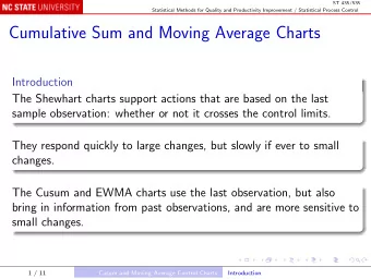
ST 435/535 Statistical Methods for Quality and Productivity Improvement / Statistical Process Control Control Charts for x and s Introduction The R chart, based on the sample range , is sensitive in detecting an assignable cause of variation
ST 435/535 Statistical Methods for Quality and Productivity Improvement / Statistical Process Control Control Charts for ¯ x and s Introduction The R chart, based on the sample range , is sensitive in detecting an assignable cause of variation that perturbs only a single value in a sample. In most other cases, the sample standard deviation s is a better measure for tracking process variability. The control charts are constructed in much the same way as for ¯ x and R . 1 / 15 Control Charts for Variables Control Charts for ¯ x and s
ST 435/535 Statistical Methods for Quality and Productivity Improvement / Statistical Process Control Construction and operation of ¯ x and s charts The ¯ x chart with three-sigma control limits: UCL = ¯ x + A 3 ¯ ¯ s Center line = ¯ ¯ x LCL = ¯ ¯ x − A 3 ¯ s . Note: S 2 is an unbiased estimator of σ 2 , but S is biased for σ . The tabulated constant A 3 is of the form √ n × 1 3 A 3 = , c 4 � � S where c 4 is the unbiasing factor: E = σ. c 4 2 / 15 Control Charts for Variables Control Charts for ¯ x and s
ST 435/535 Statistical Methods for Quality and Productivity Improvement / Statistical Process Control The s chart with three-sigma limits: UCL = B 4 ¯ s Center line = ¯ s LCL = B 3 ¯ s . As for the R chart, the control limits for the s chart are symmetric around the center line except for n ≤ 5 where B 3 would otherwise be negative: � 1 − c 2 4 B 4 = 1 + 3 , c 4 � � � 1 − c 2 4 B 3 = max 1 − 3 , 0 . c 4 3 / 15 Control Charts for Variables Control Charts for ¯ x and s
ST 435/535 Statistical Methods for Quality and Productivity Improvement / Statistical Process Control Example 6.3: inside diameters of piston rings. In R: pistonrings <- read.csv("Data/Table-06-03.csv") # convert from single-column to row-per-sample: diams <- qcc.groups(pistonrings$ID, pistonrings$Sample) # could be: diams <- with(pistonrings, qcc.groups(ID, Sample)) Begin with the s chart: summary(qcc(diams, type = "S")) 4 / 15 Control Charts for Variables Control Charts for ¯ x and s
ST 435/535 Statistical Methods for Quality and Productivity Improvement / Statistical Process Control Process variability looks stable, so continue with the ¯ x chart, specifying that the control limits are based on ¯ s (the u n w eighted ave rage of the sample s tandard d eviations): summary(qcc(diams, type = "xbar", std.dev = "UWAVE-SD")) Process mean also looks stable. 5 / 15 Control Charts for Variables Control Charts for ¯ x and s
ST 435/535 Statistical Methods for Quality and Productivity Improvement / Statistical Process Control x and s charts with variable sample size ¯ Suppose the sample sizes are n 1 , n 2 , . . . , n m , not all equal. For the center line on the ¯ x chart, just use a weighted average: � m i =1 n i ¯ x i ¯ ¯ x = . � m i =1 n i To estimate σ , use (the square root of) a pooled variance: �� m i =1 ( n i − 1) s 2 i s p = ¯ � m i =1 ( n i − 1) Note: this does not simplify to ¯ s when all n i = n . 6 / 15 Control Charts for Variables Control Charts for ¯ x and s
ST 435/535 Statistical Methods for Quality and Productivity Improvement / Statistical Process Control The ¯ x chart with three-sigma control limits: UCL = ¯ ¯ x + A 3 ¯ s p Center line = ¯ ¯ x LCL = ¯ ¯ x − A 3 ¯ s p where now A 3 varies from sample to sample. Note: the formula for A 3 is A 3 = 3 × 1 1 × √ n i c 4 where the unbiasing factor 1 / c 4 in qcc() reflects the degrees of p , � m freedom in s 2 i =1 ( n i − 1); using tables, we use n i − 1. 7 / 15 Control Charts for Variables Control Charts for ¯ x and s
ST 435/535 Statistical Methods for Quality and Productivity Improvement / Statistical Process Control For the center line on the s chart, we could use ¯ s p or the weighted average: � m i =1 n i s i s w = ¯ . � m i =1 n i Montgomery suggests using ¯ s p , but qcc() uses ¯ s w . The s chart with three-sigma limits: UCL = B 4 ˆ σ Center line = ˆ σ LCL = B 3 ˆ σ where ˆ σ is either ¯ s p or ¯ s w , and now B 3 and B 4 vary from sample to sample. 8 / 15 Control Charts for Variables Control Charts for ¯ x and s
ST 435/535 Statistical Methods for Quality and Productivity Improvement / Statistical Process Control Example 6.4: piston rings with some data excluded. In R: diamsV <- diams n <- c(5, 3, 5, 5, 5, 4, 4, 5, 4, 5, 5, 5, 3, 5, 3, 5, 4, 5, 5, 3, 5, 5, 5, 5, 5) for (i in 1:nrow(diamsV)) for (j in 1:ncol(diamsV)) if (j > n[i]) diamsV[i, j] <- NA Begin with the s chart, necessarily based on ¯ s w : summary(qcc(diamsV, type = "S")) 9 / 15 Control Charts for Variables Control Charts for ¯ x and s
ST 435/535 Statistical Methods for Quality and Productivity Improvement / Statistical Process Control Continue with the ¯ x chart, specifying that the control limits are based on ¯ s p (the r oot m ean s quare of the sample standard deviations weighted by d egrees of f reedom): summary(qcc(diamsV, type = "xbar", std.dev = "RMSDF")) Note: the default for std.dev is "UWAVE-R" , unless some n i > 25, in which case it is "RMSDF" . 10 / 15 Control Charts for Variables Control Charts for ¯ x and s
ST 435/535 Statistical Methods for Quality and Productivity Improvement / Statistical Process Control s 2 control chart As an alternative way of presenting s , we could make a chart of s 2 instead of s . The center line is just the square of either ¯ s or ¯ s p ; Montgomery s 2 appears to suggest ¯ p (“an average sample variance”). Control lines could similarly be squares of those for the s chart. But since s 2 has a χ 2 -distribution, it is more natural to specify α and use percent points χ 2 1 − α/ 2 , n − 1 and χ 2 α/ 2 , n − 1 . Of course, the square roots of those percent points could also be used on the s chart. 11 / 15 Control Charts for Variables Control Charts for ¯ x and s
ST 435/535 Statistical Methods for Quality and Productivity Improvement / Statistical Process Control Shewhart Control Chart for Individual Measurements The charts discussed above are all based on samples of size n , typically 3 to 5. In some situations, we prefer to base charts on individual measurements: n = 1. Track the process mean using the individual measurements x i . Track the process variability using the moving range : MR i = | x i − x i − 1 | . 12 / 15 Control Charts for Variables Shewhart Control Chart for Individual Measurements
ST 435/535 Statistical Methods for Quality and Productivity Improvement / Statistical Process Control Control chart for individual measurements with three-sigma limits: x + 3MR UCL = ¯ d 2 Center line = ¯ x x − 3MR LCL = ¯ . d 2 Control chart for moving range is the same as the R chart. 13 / 15 Control Charts for Variables Shewhart Control Chart for Individual Measurements
ST 435/535 Statistical Methods for Quality and Productivity Improvement / Statistical Process Control Example 6.5: Loan processing costs In R: qcc() does not make a moving range chart, so we construct a matrix with overlapping samples of n = 2: mortgage <- read.csv("Data/Table-06-06.csv") nr <- nrow(mortgage) mortgagePairs <- with(mortgage, cbind(Cost[1:(nr-1)], Cost[2:nr])) summary(qcc(mortgagePairs, type = "R")) Montgomery: “the moving range chart cannot really provide useful information about a shift in process variability.” 14 / 15 Control Charts for Variables Shewhart Control Chart for Individual Measurements
ST 435/535 Statistical Methods for Quality and Productivity Improvement / Statistical Process Control Continue with the x chart: summary(qcc(mortgage$Cost, type = "xbar.one")) Note: the default control limits use the moving range of k = 2 values. That can be over-ridden: summary(qcc(mortgage$Cost, type = "xbar.one", std.dev = sd.xbar.one(mortgage$Cost, k = 3))) 15 / 15 Control Charts for Variables Shewhart Control Chart for Individual Measurements
Recommend
More recommend
Explore More Topics
Stay informed with curated content and fresh updates.
