Contents 1 Introduction 1 2 The Radon Study 2 3 Organizing - PDF document

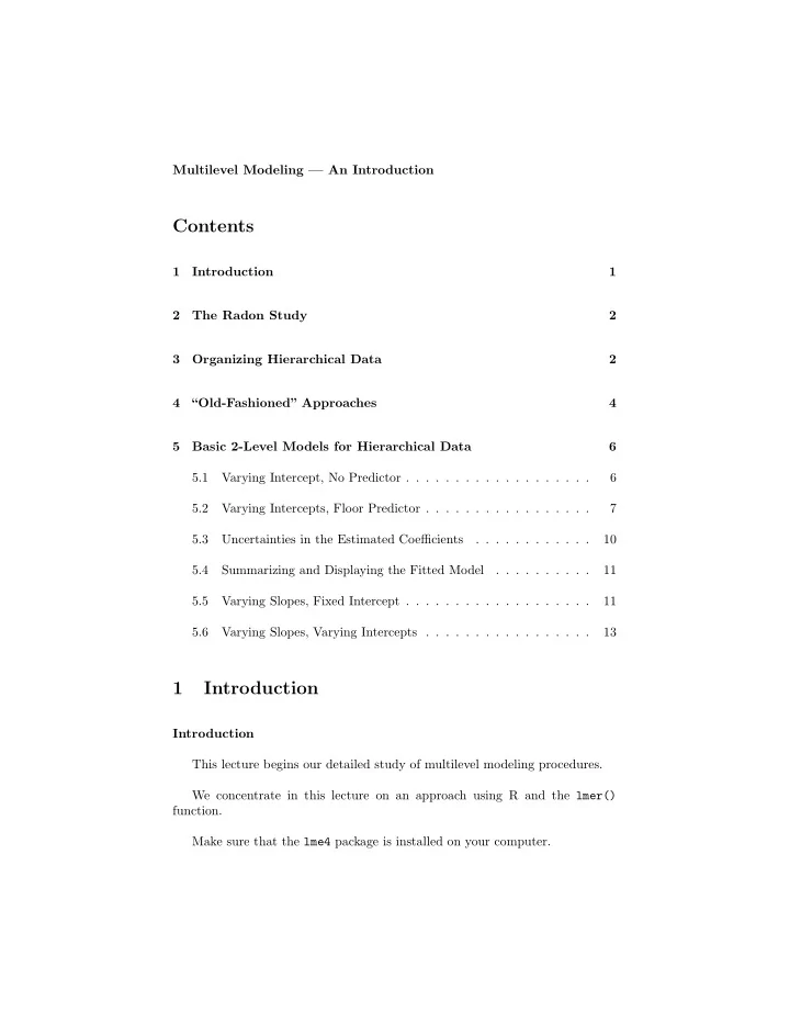
Multilevel Modeling — An Introduction Contents 1 Introduction 1 2 The Radon Study 2 3 Organizing Hierarchical Data 2 4 “Old-Fashioned” Approaches 4 5 Basic 2-Level Models for Hierarchical Data 6 5.1 Varying Intercept, No Predictor . . . . . . . . . . . . . . . . . . . 6 5.2 Varying Intercepts, Floor Predictor . . . . . . . . . . . . . . . . . 7 5.3 Uncertainties in the Estimated Coefficients . . . . . . . . . . . . 10 5.4 Summarizing and Displaying the Fitted Model . . . . . . . . . . 11 5.5 Varying Slopes, Fixed Intercept . . . . . . . . . . . . . . . . . . . 11 5.6 Varying Slopes, Varying Intercepts . . . . . . . . . . . . . . . . . 13 1 Introduction Introduction This lecture begins our detailed study of multilevel modeling procedures. We concentrate in this lecture on an approach using R and the lmer() function. Make sure that the lme4 package is installed on your computer.

2 The Radon Study The Radon Study One of the introductory examples in Gelman & Hill , and our first example of multilevel modeling, concerns the level of radon gas in houses in Minnesota. Radon is a carcinogen estimated to cause several thousand lung cancer deaths per year in the U.S. The Radon Study The distribution of radon in American houses varies greatly. Some houses have dangerously high concentrations. The EPA did a study of 80,000 houses throughout the country, in order to better understand the distribution of radon. Two important predictors were available: • Whether the measurement was taken in the basement, or the first floor, and • The level of uranium in the county Higher levels of uranium are expected to lead to higher radon levels, in general. And, in general, more radon will be measured in the basement than on the first floor. 3 Organizing Hierarchical Data Hierarchical Data The data are organized hierarchically in the radon study. Houses are situated within 85 counties. Each house has a radon level that is the outcome variable in the study, and a binary floor indicator (0 for basement, 1 for first floor) which is a potential predictor. Uranium levels are measured at the county level. There are 85 counties, and for each one a uranium background level is available. 2

We say that the level-1 data is at the house level, and the level-2 data is at the county level. Houses are grouped within counties. Organizing Hierarchical Data There are a number of ways to organize hierarchical data, and a number of different ways to write the same hierarchical model. One method breaks the data down by levels, and links the data through an intermediary variable. This method offers some important advantages. It saves some space, and it emphasizes the hierarchical structure of the data. Two Files for Two Levels The level-1 file looks like this. county radon floor 1 1 2.2 1 2 1 2.2 0 3 1 2.9 0 4 1 1.0 0 5 2 3.1 0 6 2 2.5 0 7 2 1.5 0 . . . . . . . . 917 84 5.0 0 918 85 3.7 0 919 85 2.9 0 Two Files for Two Levels The level-2 file looks like this county uranium 1 1 -0.689047595 2 2 -0.847312860 3 3 -0.113458774 . . . . . . 85 85 0.355286981 3

A Single File for All Levels An alternative, less efficient file structure puts all the data in the same file. By necessity, some data are redundant. The full data file looks like this: radon floor uranium county 1 0.78845736 1 -0.689047595 1 2 0.78845736 0 -0.689047595 1 3 1.06471074 0 -0.689047595 1 4 0.00000000 0 -0.689047595 1 5 1.13140211 0 -0.847312860 2 6 0.91629073 0 -0.847312860 2 . . . . . . . . . . 917 1.60943791 0 -0.090024275 84 918 1.30833282 0 0.355286981 85 919 1.06471074 0 0.355286981 85 4 “Old-Fashioned” Approaches “Old-Fashioned” Approaches We have potential sources of variation at the county level, and at the house level. There are a number of potential approaches to analyzing such data that people have used prior to the popularization of multilevel modeling. Two such approaches, discussed by Gelman & Hill , are • Complete Pooling. Completely ignore the fact that the relationship be- tween radon and uranium might vary across counties, and simply pool all the data. This model is y i = α + βx i + ǫ i (1) • No Pooling. Include county as a categorical predictor in the model, thereby adding 85 county indicators to the model. y i = α j [ i ] + βx i + ǫ i (2) 4

Fitting the Complete-Pooling Regression First, we fit the complete-pooling model: read.table ("radon.txt",header=TRUE) > radon.data ← > attach (radon.data) ← lm (radon ˜ floor ) > complete.pooling > display ( complete.pooling ) lm(formula = radon ~ floor) coef.est coef.se (Intercept) 1.33 0.03 floor -0.61 0.07 --- n = 919, k = 2 residual sd = 0.82, R-Squared = 0.07 Fitting the No-Pooling Regression ← lm (radon ˜ floor + factor (county)-1) > no.pooling > display (no.pooling) lm(formula = radon ~ floor + factor(county) - 1) coef.est coef.se floor -0.72 0.07 factor(county)1 0.84 0.38 factor(county)2 0.87 0.10 factor(county)3 1.53 0.44 . . . . . . factor(county)84 1.65 0.21 factor(county)85 1.19 0.53 --- n = 919, k = 86 residual sd = 0.76, R-Squared = 0.77 5

5 Basic 2-Level Models for Hierarchical Data Basic 2-Level Models At level 1, we have floor as a potential predictor of radon level. We can think of the linear regression relating floor to radon in very simple terms. The y -intercept is the average radon value at in the basement, i.e., when floor = 0 . The slope is the difference between average radon levels in the basement and first floor. There are a number of ways we could model the situation. Basic 2-Level Models Our data are organized within county. Even in such a simple situation, there are numerous potential models for the relationship between radon level and floor. • The slopes could vary across counties • The intercepts could vary across counties • Both the slopes and intercepts could vary Gelman & Hill introduce a notation we can familiarize ourselves with, al- though it will take a little effort getting used to. Let’s diagram these basic models and write them in the Gelman & Hill “full data” notation. 5.1 Varying Intercept, No Predictor Varying Intercepts, No Predictor One model allows the intercepts to vary across county, and uses no predictors. This model, which is formally equivalent to a one way random-effects ANOVA, can be written as y i = α j [ i ] + ǫ i (3) 6

with ǫ i ∼ N(0 , σ 2 y ) (4) and α j [ i ] ∼ N( µ α , σ 2 α ) (5) In the above notation, “ j [ i ]” means “the value of j assigned to the ith unit.” Varying Intercepts, No Predictor ← lmer (radon ˜ 1 + (1 | county )) > M0 > display (M0) lmer(formula = radon ~ 1 + (1 | county)) coef.est coef.se 1.31 0.05 Error terms: Groups Name Std.Dev. county (Intercept) 0.31 Residual 0.80 --- number of obs: 919, groups: county, 85 AIC = 2265.4, DIC = 2251 deviance = 2255.2 5.2 Varying Intercepts, Floor Predictor Varying Intercepts, Floor Predictor The next model adds the floor predictor, and keeps varying intercepts. This model can be written as y i = α j [ i ] + βx i + ǫ i (6) with α j [ i ] ∼ N( µ α , σ 2 α ) (7) This model looks much like the “no-pooling” model we looked at before, except that the earlier model used least squares estimation and essentially set each α to the value obtained by fitting regression within a county. Multilevel modeling uses a simultaneous estimation approach that is more sophisticated at dealing with large differences in sample size across counties. 7

Varying Intercepts, Floor Predictor Here is a picture of the model with 5 counties: Varying Intercepts, Floor Predictor Here is how we fit this model using R. > M1 ← lmer (radon ˜ floor + (1 | county )) > display (M1) lmer(formula = radon ~ floor + (1 | county)) coef.est coef.se (Intercept) 1.46 0.05 floor -0.69 0.07 Error terms: Groups Name Std.Dev. county (Intercept) 0.33 Residual 0.76 --- number of obs: 919, groups: county, 85 AIC = 2179.3, DIC = 2156 deviance = 2163.7 Varying Intercepts, Floor Predictor This model displays fixed and random effect results. To see more detail, we can use the summary() function. > summary (M1) 8

Linear mixed model fit by REML Formula: radon ~ floor + (1 | county) AIC BIC logLik deviance REMLdev 2179 2199 -1086 2164 2171 Random effects: Groups Name Variance Std.Dev. county (Intercept) 0.108 0.328 Residual 0.571 0.756 Number of obs: 919, groups: county, 85 Fixed effects: Estimate Std. Error t value (Intercept) 1.4616 0.0516 28.34 floor -0.6930 0.0704 -9.84 Correlation of Fixed Effects: (Intr) floor -0.288 Note that the average intercept is 1.46, but the intercepts, across counties, have a standard deviation of σ α = 0 . 33. Varying Intercepts, Floor Predictor We can call for estimates of the county level coefficients: > coef (M1) $county (Intercept) floor 1 1.1915015 -0.6929905 2 0.9276037 -0.6929905 ... 83 1.5716904 -0.6929905 84 1.5906371 -0.6929905 85 1.3862299 -0.6929905 We can examine the fixed and random effects separately: > f i x e f (M1) (Intercept) floor 1.462 -0.693 9