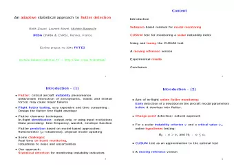
Content Variations on CUSUM tests for flutter monitoring - PowerPoint PPT Presentation
Content Variations on CUSUM tests for flutter monitoring Introduction Mich` ele Basseville, Laurent Mevel, Rafik Zouari Subspace-based residual for modal monitoring IRISA (CNRS & INRIA), Rennes, France CUSUM test for monitoring a scalar
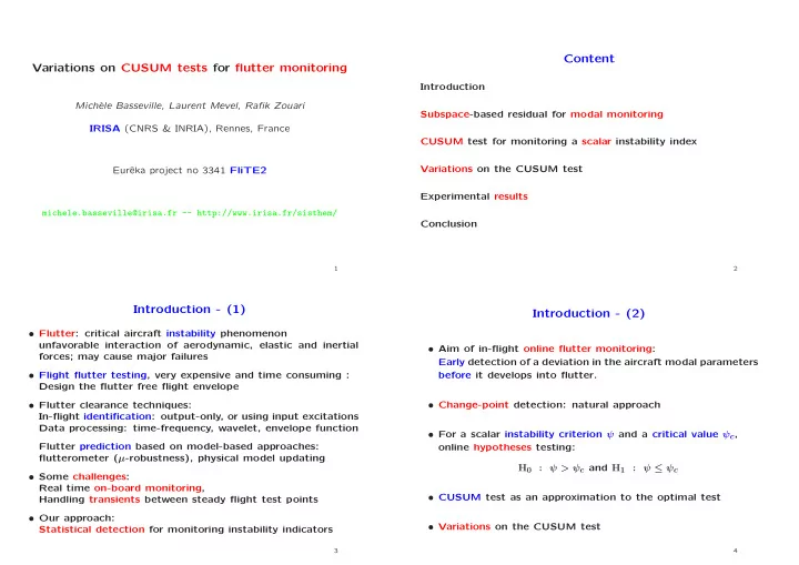
Content Variations on CUSUM tests for flutter monitoring Introduction Mich` ele Basseville, Laurent Mevel, Rafik Zouari Subspace-based residual for modal monitoring IRISA (CNRS & INRIA), Rennes, France CUSUM test for monitoring a scalar instability index Variations on the CUSUM test Eurˆ eka project no 3341 FliTE2 Experimental results michele.basseville@irisa.fr -- http://www.irisa.fr/sisthem/ Conclusion 1 2 Introduction - (1) Introduction - (2) • Flutter: critical aircraft instability phenomenon unfavorable interaction of aerodynamic, elastic and inertial • Aim of in-flight online flutter monitoring: forces; may cause major failures Early detection of a deviation in the aircraft modal parameters • Flight flutter testing, very expensive and time consuming : before it develops into flutter. Design the flutter free flight envelope • Flutter clearance techniques: • Change-point detection: natural approach In-flight identification: output-only, or using input excitations Data processing: time-frequency, wavelet, envelope function • For a scalar instability criterion ψ and a critical value ψ c , Flutter prediction based on model-based approaches: online hypotheses testing: flutterometer ( µ -robustness), physical model updating H 0 : ψ > ψ c and H 1 : ψ ≤ ψ c • Some challenges: Real time on-board monitoring, • CUSUM test as an approximation to the optimal test Handling transients between steady flight test points • Our approach: • Variations on the CUSUM test Statistical detection for monitoring instability indicators 3 4
Λ modes θ ∆ Subspace-based residual for modal monitoring Canonical parameter : = vec Φ mode shapes Φ X k +1 = F X k + V k F φ λ = λ φ λ Φ∆ O p +1 ( θ ) = Observability in modal basis : . . . ∆ Φ∆ p Y k = H X k ϕ λ = H φ λ Given: R 0 R 1 R 2 . . . � � R 1 R 2 R 3 . . . H ⋆ ∆ ∆ • a reference parameter θ ⋆ , by SVD of � Y k Y T p +1 ,q (reference data) H R i = E , = k − i R 2 R 3 R 4 . . . . . ... . . . . . . . U ( θ ⋆ ) T H ⋆ � p +1 ,q = 0 parameter estimating function R i = H F i G = ⇒ H = O C U ( θ ⋆ ) T O p +1 ( θ ⋆ ) = 0 , U ( θ ⋆ ) T U ( θ ⋆ ) = I � G H � C ∆ F 2 G = F G . . . HF O ∆ = , • a n -size sample of new data; H p +1 ,q � HF 2 � � G ∆ X k Y T . = E . . k For testing θ = θ ⋆ , statistics (residual) : Output-only covariance-driven subspace identification = √ n vec � � ζ n ( θ ⋆ ) ∆ U ( θ ⋆ ) T H p +1 ,q � SVD of H − → O − → ( H, F ) − → ( λ, ϕ λ ) 5 6 Local approach to testing H 1 : θ = θ ⋆ + Υ / √ n Data-driven computation for online detection � � H 0 : θ = θ ⋆ and n − p k = q Z k ( θ ⋆ ) / √ n Mean sensitivity and covariance matrices: � ζ n ( θ ⋆ ) = = 1 / √ n ∂/∂ ˜ � � � J n ( θ ⋆ , θ ) ∆ � θ = θ ⋆ , Σ n ( θ ⋆ , θ ) ∆ ζ n ( θ ⋆ ) ζ n ( θ ⋆ ) T θ E θ ζ n (˜ θ ) � = E θ � � ˜ � � T Y + Z k ( θ ⋆ ) ∆ k,p +1 Y − T = K k ( θ ⋆ , θ ) vec U ( θ ⋆ ) k,q If Σ n ( θ ⋆ , θ ) is positive definite, and for all Υ , under both hypoth: Σ n ( θ ⋆ , θ ) − 1 / 2 ( ζ n ( θ ⋆ ) − J n ( θ ⋆ , θ ) Υ) Another approximation → N (0 , I ) n → ∞ For n large enough, and k = 1 , . . . , n , Normalized residual: Z k ( θ ⋆ ) ≈ Gaussian i.i.d., mean 0 before change and � = 0 after. ζ n ( θ ⋆ ) ∆ = K n ( θ ⋆ , θ ) ζ n ( θ ⋆ ) K n ( θ ⋆ , θ ) ∆ , Σ n ( θ ⋆ , θ ) ∆ = Σ − 1 / 2 J T n Σ − 1 = J T n Σ − 1 n J n Monitoring any function ψ ( θ ) n n Replace J n ( θ ⋆ , θ ) with J n ( θ ⋆ , θ ) J ⋆ θψ , where J ⋆ θψ = ∂θ/∂ψ | θ = θ ⋆ . � � ζ n ( θ ⋆ ) − Σ n ( θ ⋆ , θ ) 1 / 2 Υ → N (0 , I ) n → ∞ 7 8
CUSUM test for monitoring a scalar index The crossing of a critical ψ c by ψ is reflected into a change with the same sign in the mean ν of the i.i.d. Gaussian Z k ( θ ⋆ ) . Variations on the CUSUM test - (1) The CUSUM test may be used for testing between: H 1 : ν ≤ 0 H 0 : ν > 0 and For detecting aircraft instability precursors, select: Procedure for unknown sign and magnitude of change in ψ : An instability criterion ψ and a critical value ψ c ; a) i) Set a min. change magnitude ν m > 0 , and test between: H 0 : ν > ν m / 2 and H 1 : ν ≤ − ν m / 2 b) A left kernel matrix U ( . ) ; n − p S n ( θ ⋆ ) ∆ k = q ( Z k ( θ ⋆ ) + ν m ) , T n ( θ ⋆ ) ∆ � = = k = q,...,n − p S k ( θ ⋆ ) max A reference θ ⋆ for estimating J n ( θ ⋆ ) and Σ − 1 c) n ( θ ⋆ ) ; H 1 g n ( θ ⋆ ) ∆ > = T n ( θ ⋆ ) − S n ( θ ⋆ ) < ̺ threshold d) A min. change magnitude ν m and a threshold ̺ . H 0 ii) Run 2 tests in parallel, for decreasing and increasing ψ ; iii) Make a decision from the first test which fires; iv) Reset all sums and extrema to 0, switch to the other test. 9 10 Solution 2. - Details Variations on the CUSUM test - (2) i) Compute the critical eigenvalues λ c at flight point t using identified modal signatures ( θ 1 , . . . , θ t ) Three solutions for b)-c): and extrapolation of the characteristic polynomial associated with the quasi-steady aeroelastic model 1. θ ⋆ ∆ q + ( K + V 2 C ) q = 0 ; = θ 0 identified on reference data for the stable system; M ¨ q + ( D + V B ) ˙ U ( θ ⋆ ) computed, J n ( θ 0 ) , Σ − 1 ii) Build the critical modal signature θ c from λ c and n ( θ 0 ) estimated recursively with the test data. the mode-shapes ϕ λ identified at flight point t ; 2. θ ⋆ ∆ = θ c , critical parameter closer to instability, computed iii) Compute the Z k ( θ c ) ’s and S n ( θ c ) ; at each flight point using θ 0 and an aeroelastic model; Σ − 1 J n ( θ c ) and ˆ ˆ Compute n ( θ c ) with the test data; U ( θ ⋆ ) computed, J n ( θ c ) , Σ − 1 n ( θ c ) estimated recursively with the test data. iv) Run the CUSUM test between flight points t and t + 1 ; v) Repeat these steps for flight point t + 1 : 3. U ( . ) ∆ � = U n estimated on test data, modal identification of θ t +1 to update the prediction of θ c , J n ( θ 0 ) , Σ − 1 n ( θ 0 ) estimated recursively with the test data. J n ( θ c ) and ˆ ˆ Σ − 1 computation of n ( θ c ) , CUSUM test between t + 1 and t + 2 . 11 12
Solution 3. - Details Solution 3. - Details (Contd.) i) Initialization For an initial airspeed: ˆ J n ; Estimate a reference θ 0 and compute the constant terms in Select data sample size L , lag τ , block size K , ν m , and ̺ ; Σ − 1 Compute ˆ ˆ J L + τ with the first L + τ samples; L + τ and Compute ˆ U L + τ with ( Y 1 , ..., Y L ) ; Compute the Z k ’s and S L + τ . ii) Recursive loop Running the CUSUM test: for each n ≥ L + τ : � Compute recursively U n with ( Y n − τ − L +1 , ..., Y n − τ ) ; Σ − 1 � � J n to compute S n and g n until g n ≥ ̺ . � Use U n with and n Σ − 1 � J n every K samples. � Update recursively and n 13 14 Example - Aeroelastic Hancock wing model Example - Numerical results Rigid wing with constant chord; 2 d.o.f. in bending and torsion. CUSUM test run with ν m = 0 . 1 , ̺ = 100 , and the damping as ψ . J n , ˆ ˆ Solution 1. with θ ⋆ = θ 0 at V = 20 m/s , online recursive Σ n . J n , ˆ ˆ Matrix F , and eigenvalues λ : functions of airspeed V . Solution 2. with θ ⋆ = θ c at V = 85 m/s , online recursive Σ n . Solution 3. with online recursive ˆ U n , ˆ J n , ˆ Flutter airspeed: V f = 88 . 5 m/s . Σ n . Stability indicator ψ : Damping coefficient Alarm onset times depend on threshold; ˆ V f is more important. Modal frequencies variation with airspeed Modal damping coefficients variation with airspeed 0.2 13 Solution 1. θ ⋆ far from instability, alarm at V =67 m/s , ˆ V f =65 m/s . Bending mode Bending mode Torsional mode Torsional mode 12 0.15 The test detects that torsional damping decreases under ψ c . Damping coefficient 11 0.1 F(Hz) 10 0.05 Solution 2. θ ⋆ close to instability, alarm at V =88 m/s , ˆ 9 V f =85 m/s . 0 8 The test detects that flutter is happening between two steady 7 −0.05 0 10 20 30 40 50 60 70 80 90 0 10 20 30 40 50 60 70 80 88.5 V(m/s) V(m/s) points, and confirms the flutter prediction. Frequencies Damping coefficients Solution 3. Alarm at V =88 m/s , ˆ V f =78 m/s much closer to flutter. Bending & torsion modes Good behavior for light damping decrease before alarm. 20700 -size 2D-samples simulated (300 for each V =20:1:88 m/s ). Detection (before flutter) of torsional damping drop. 15 16
Recommend
More recommend
Explore More Topics
Stay informed with curated content and fresh updates.
