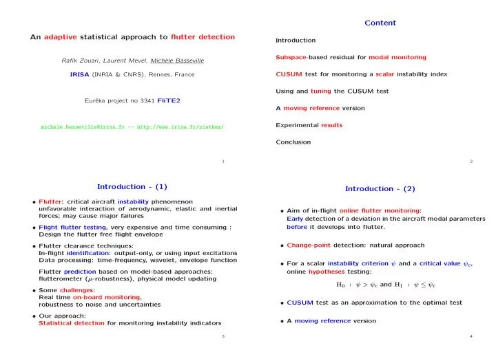
Content An adaptive statistical approach to flutter detection - PowerPoint PPT Presentation

Content An adaptive statistical approach to flutter detection Introduction Subspace-based residual for modal monitoring Rafik Zouari, Laurent Mevel, Mich` ele Basseville IRISA (INRIA & CNRS), Rennes, France CUSUM test for monitoring a scalar instability index Using and tuning the CUSUM test Eurˆ eka project no 3341 FliTE2 A moving reference version Experimental results michele.basseville@irisa.fr -- http://www.irisa.fr/sisthem/ Conclusion 1 2 Introduction - (1) Introduction - (2) • Flutter: critical aircraft instability phenomenon unfavorable interaction of aerodynamic, elastic and inertial • Aim of in-flight online flutter monitoring: forces; may cause major failures Early detection of a deviation in the aircraft modal parameters • Flight flutter testing, very expensive and time consuming : before it develops into flutter. Design the flutter free flight envelope • Change-point detection: natural approach • Flutter clearance techniques: In-flight identification: output-only, or using input excitations Data processing: time-frequency, wavelet, envelope function • For a scalar instability criterion ψ and a critical value ψ c , Flutter prediction based on model-based approaches: online hypotheses testing: flutterometer ( µ -robustness), physical model updating H 0 : ψ > ψ c and H 1 : ψ ≤ ψ c • Some challenges: Real time on-board monitoring, • CUSUM test as an approximation to the optimal test robustness to noise and uncertainties • Our approach: • A moving reference version Statistical detection for monitoring instability indicators 3 4

  Λ modes θ ∆ Subspace-based residual for modal monitoring   Canonical parameter : =     vec Φ mode shapes   Φ   X k +1 = F X k + V k F φ λ = λ φ λ        Φ∆      O p +1 ( θ ) =    Observability in modal basis : .   .  .         ∆ Φ∆ p    Y k = H X k ϕ λ = H φ λ     Given: R 0 R 1 R 2 . . .       R 1 R 2 R 3 . . . � � • a reference parameter θ ⋆ , by SVD of ˆ H ⋆   ∆ Y k Y T ∆ p +1 ,q (reference data)   R i = E , H =   k − i   R 2 R 3 R 4 . . .      . . .  ... . . .   . . . U ( θ ⋆ ) T H ⋆ ˆ p +1 ,q = 0 parameter estimating function R i = H F i G = ⇒ H = O C U ( θ ⋆ ) T O p +1 ( θ ⋆ ) = 0 , U ( θ ⋆ ) T U ( θ ⋆ ) = I   � G H � C ∆ F 2 G   = F G . . .   HF   O ∆   = , • a n -size sample of new data; ˆ   H p +1 ,q HF 2   � �   G ∆ X k Y T  .  = E . . k For testing θ = θ ⋆ , statistics (residual) : Output-only covariance-driven subspace identification = √ n vec � � ζ n ( θ ⋆ ) ∆ U ( θ ⋆ ) T ˆ H p +1 ,q SVD of H − → O − → ( H, F ) − → ( λ, ϕ λ ) 5 6 Local approach to testing Data-driven computation for online detection H 1 : θ = θ ⋆ + Υ / √ n � � H 0 : θ = θ ⋆ and n − p k = q Z k ( θ ⋆ ) / √ n � ζ n ( θ ⋆ ) ≈ Mean sensitivity and covariance matrices: = 1 / √ n ∂/∂ ˜ � � � J n ( θ ⋆ , θ ) ∆ θ = θ ⋆ , Σ n ( θ ⋆ , θ ) ∆ θ E θ ζ n (˜ � ζ n ( θ ⋆ ) ζ n ( θ ⋆ ) T θ ) � = E θ � � ˜ � � T Y + k,p +1 Y − T Z k ( θ ⋆ ) ∆ = K k ( θ ⋆ , θ ) vec U ( θ ⋆ ) k,q If Σ n ( θ ⋆ , θ ) is positive definite, and for all Υ , under both hypoth: Σ n ( θ ⋆ , θ ) − 1 / 2 ( ζ n ( θ ⋆ ) − J n ( θ ⋆ , θ ) Υ) → N (0 , I ) Another approximation n → ∞ Normalized residual: For n large enough, and k = 1 , . . . , n , ζ n ( θ ⋆ ) ∆ = K n ( θ ⋆ , θ ) ζ n ( θ ⋆ ) Z k ( θ ⋆ ) ≈ Gaussian i.i.d., mean 0 before change and � = 0 after. K n ( θ ⋆ , θ ) ∆ = Σ − 1 / 2 n Σ − 1 , Σ n ( θ ⋆ , θ ) ∆ n Σ − 1 J T = J T n J n n n Monitoring any function ψ ( θ ) Replace J n ( θ ⋆ , θ ) with J n ( θ ⋆ , θ ) J ⋆ θψ , where J ⋆ � � θψ = ∂θ/∂ψ | θ = θ ⋆ . ζ n ( θ ⋆ ) − Σ n ( θ ⋆ , θ ) 1 / 2 Υ → N (0 , I ) n → ∞ 7 8

CUSUM test for monitoring a scalar index Using and tuning the CUSUM test The crossing of a critical ψ c by ψ is reflected into a change with the same sign in the mean ν of the i.i.d. Gaussian Z k ( θ ⋆ ) . For detecting aircraft instability precursors, select: The CUSUM test may be used for testing between: H 1 : ν ≤ 0 a) An instability criterion ψ and a critical value ψ c ; H 0 : ν > 0 and b) A left kernel matrix U ( . ) ; Procedure for unknown sign and magnitude of change in ψ c) Estimates of J n ( θ ⋆ , θ ) and Σ n ( θ ⋆ , θ ) ; i) Set a min. change magnitude ν m > 0 , and test between: d) A min. change magnitude ν m and a threshold ̺ . H 0 : ν > ν m / 2 and H 1 : ν ≤ − ν m / 2 Two solutions for b)-c): n − p S n ( θ ⋆ ) ∆ k = q ( Z k ( θ ⋆ ) + ν m ) , T n ( θ ⋆ ) ∆ � = = k = q,...,n − p S k ( θ ⋆ ) max 1. θ ⋆ ∆ = θ 0 identified on reference data for the stable system; U ( θ ⋆ ) computed, J n , Σ n estimated once for all with those data. H 1 g n ( θ ⋆ ) ∆ > = T n ( θ ⋆ ) − S n ( θ ⋆ ) < ̺ threshold H 0 2. U ( . ) ∆ = ˆ U n estimated on test data; ii) Run 2 tests in parallel, for decreasing and increasing ψ ; iii) Make a decision from the first test which fires; J n , Σ n estimated recursively with those test data. iv) Reset all sums and extrema to 0, switch to the other test. 9 10 Example - Aeroelastic Hancock wing model The moving reference version Rigid wing with constant chord; 2 d.o.f. in bending and torsion. Matrix F , and eigenvalues λ : functions of airspeed V . Flutter airspeed: V f = 88 . 5 m/s . Stability indicator: Damping coefficient Modal frequencies variation with airspeed Modal damping coefficients variation with airspeed 13 0.2 Bending mode Bending mode Torsional mode Torsional mode 12 0.15 11 Damping coefficient 0.1 F(Hz) 10 0.05 9 0 8 7 −0.05 0 10 20 30 40 50 60 70 80 90 0 10 20 30 40 50 60 70 80 88.5 V(m/s) V(m/s) Frequency Damping coefficient 20700 -size 2D-samples simulated (300 for each V =20:1:88 m/s ). 11 12

CUSUM test for the bending damping coefficient CUSUM test for the torsional damping coefficient Example - Numerical results 100 100 80 80 CUSUM test run with ν m = 0 . 1 , ̺ = 100 , and the damping as ψ . 60 60 40 40 Solution 1. with θ ⋆ = θ 0 at V = 20 m/s and fixed J , Σ . 20 20 Solution 2. with online ˆ U n , ˆ J n , ˆ 0 0 Σ n . 20 30 40 50 60 70 80 85 88 20 30 40 50 60 70 80 85 88 V(m/s) (300 samples for each 1m/s) V(m/s) (300 samples for each 1m/s) Solution 1: Bending mode Solution 1: Torsion mode Solution 1. θ ⋆ far from instability, too early alarm at V =69 m/s . CUSUM test with moving reference for the bending damping coefficient CUSUM test with moving reference for the torsional damping coefficient 100 100 The test detects that torsional damping decreases under the predefined threshold. 80 80 60 60 Solution 2. Alarm at V = 82 m/s much closer to flutter. 40 40 The test detects that the torsional damping decreases abruptly. 20 20 0 0 20 30 40 50 60 70 80 85 88 20 30 40 50 60 70 80 85 88 Both algorithms do what they are intended to do. V(m/s) (300 samples for each 1m/s) V(m/s) (300 samples for each 1m/s) Solution 2: Bending mode Solution 2: Torsion mode Only Solution 2 is a flutter detection algorithm. 13 14 Conclusion Online detection of instability precursors Model-free subspace statistics, local approach, CUSUM Analytical model for flutter prediction Recursive computation of covariance matrix Relevance on a small simulated structure Limitations: cost of online kernel and covariance computation Major issues: dimension of θ , large number of correlated criteria 15