Constraint Satisfaction Problems Chapter 6 Outline Topics: CSP - PowerPoint PPT Presentation
Constraint Satisfaction Problems Chapter 6 Outline Topics: CSP examples Backtracking search for CSPs Improving backtracking efficiency Problem structure and problem decomposition Local search for CSPs Constraint satisfaction
Constraint Satisfaction Problems Chapter 6
Outline Topics: • CSP examples • Backtracking search for CSPs • Improving backtracking efficiency • Problem structure and problem decomposition • Local search for CSPs
Constraint satisfaction problems (CSPs) Standard search problem: • A state is a “black box” – can be any data structure that supports goal test, eval, successor
Constraint satisfaction problems (CSPs) Standard search problem: • A state is a “black box” – can be any data structure that supports goal test, eval, successor CSP: • Each state has some structure, given by a set of variables and a set of constraints . • The problem is solved when each variable has a value that satisfies the constraints. • In a CSP, can use general purpose algorithms (as opposed to the problem-specific heuristics that we’ve seen in search).
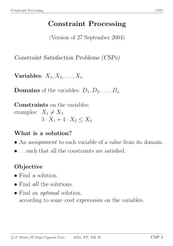
Constraint satisfaction problems (CSPs) CSP: • Defined by a set of variables X 1 , . . . , X n , and a set of constraints C 1 , . . . , C m . • Each variable X i has an associated domain D i . • Each constraint C i involves some subset of the variables and specifies allowable combinations of values for that subset. • A state is an assignment to some or all of the variable. • A solution is a complete assignment that satisfies all constraints. (Sometimes: maximize an objective function .)
CSPs continued • This is a simple example of a formal representation language • Allows useful general-purpose algorithms with more power than standard search algorithms
Example: Map-Coloring Northern Territory Western Queensland Australia South Australia New South Wales Victoria Tasmania
Example: Map-Coloring Northern Territory Western Queensland Australia South Australia New South Wales Victoria Tasmania Variables WA , NT , Q , NSW , V , SA , T Domains D i = { red , green , blue } Constraints : adjacent regions must have different colours • e.g., WA � = NT (if the language allows this), or • ( WA , NT ) ∈ { ( red , green ) , ( red , blue ) , ( green , red ) , . . . }
Example: Map-Coloring contd. Northern Territory Western Queensland Australia South Australia New South Wales Victoria Tasmania Solutions are assignments satisfying all constraints, e.g., { WA = red , NT = green , Q = red , NSW = green , V = red , SA = blue , T = green }
Constraint graph • Binary CSP : Each constraint relates at most two variables • Constraint graph : Nodes are variables, arcs show constraints NT Q WA SA NSW V Victoria T • General-purpose CSP algorithms use the graph structure to speed up search. • E.g., Tasmania is an independent subproblem!
Varieties of CSPs Discrete variables, finite domains: ⇒ O ( d n ) complete assignments • n vars, domain size d = • e.g., Boolean CSPs, incl. Boolean satisfiability (NP-complete)
Varieties of CSPs Discrete variables, finite domains: ⇒ O ( d n ) complete assignments • n vars, domain size d = • e.g., Boolean CSPs, incl. Boolean satisfiability (NP-complete) Discrete variables, infinite domains: • integers, strings, etc. • e.g., job scheduling, variables are start/end days for each job. ⇒ need a constraint language e.g., StartJob 1 + 5 ≤ StartJob 3 • linear constraints solvable; nonlinear undecidable.
Varieties of CSPs Discrete variables, finite domains: ⇒ O ( d n ) complete assignments • n vars, domain size d = • e.g., Boolean CSPs, incl. Boolean satisfiability (NP-complete) Discrete variables, infinite domains: • integers, strings, etc. • e.g., job scheduling, variables are start/end days for each job. ⇒ need a constraint language e.g., StartJob 1 + 5 ≤ StartJob 3 • linear constraints solvable; nonlinear undecidable. Continuous variables: • e.g., start/end times for Hubble Telescope observations. • linear constraints solvable in poly time by LP methods.
Varieties of Constraints Unary constraints: Involve a single variable. • e.g., SA � = green
Varieties of Constraints Unary constraints: Involve a single variable. • e.g., SA � = green Binary constraints: Involve pairs of variables. • e.g., SA � = WA
Varieties of Constraints Unary constraints: Involve a single variable. • e.g., SA � = green Binary constraints: Involve pairs of variables. • e.g., SA � = WA Higher-order constraints: Involve 3 or more variables. • e.g., sudoku, cryptarithmetic column constraints
Varieties of Constraints Unary constraints: Involve a single variable. • e.g., SA � = green Binary constraints: Involve pairs of variables. • e.g., SA � = WA Higher-order constraints: Involve 3 or more variables. • e.g., sudoku, cryptarithmetic column constraints Preferences (soft constraints): • e.g., red is better than green • Often representable by a cost for each variable assignment. → constrained optimization problems
Higher-Order Example: Cryptarithmetic T W O O F T U W R + T W O F O U R X 3 X 2 X 1 • Variables : F T U W R O X 1 X 2 X 3 • Domains : { 0 , 1 , 2 , 3 , 4 , 5 , 6 , 7 , 8 , 9 } • Constraints (represented by square boxes): • alldiff ( F , T , U , W , R , O ) • O + O = R + 10 · X 1 , etc.
Higher-order Constraints Higher-order constraints can be reduced to binary constraints by introducing new auxiliary variables. • We’re not going to cover this. • See Exercise 6.6, 3 rd ed. or Exercise 5.11, 2 nd ed. for a hint as to how this can be done. • But as a result of this, we’ll just deal with binary constraints.
Real-world CSPs • Assignment problems e.g., who teaches what class • Timetabling problems e.g., which class is offered when and where? • Hardware configuration • Transportation scheduling • Factory scheduling • Floorplanning Notice that many real-world problems involve real-valued ☞ variables.
Naive Search Formulation (Incremental) • We start with the straightforward, dumb approach, then fix it • Define the state-space: States are defined by the values assigned so far. Initial state: The empty assignment, ∅ Successor function: Assign a value to an unassigned variable that does not conflict with current assignment. • Fail if no legal assignments (not fixable!) Goal test: The current assignment is complete
Naive Search Formulation (Incremental) Notes: 1 This can be used for all CSPs! 2 Every solution appears at depth n with n variables • use depth-first search 3 Path is irrelevant 4 b = ( n − ℓ ) d at depth ℓ where domain size for all variables is d . • there are n ! d n leaves, even though there are only d n complete assignments!
Backtracking Search • Problem with the naive formulation: • It ignores that variable assignments are commutative • i.e. [ WA = red then NT = green ] same as [ NT = green then WA = red ] • So just consider assignments to a single variable at each node • Obtain d n leaves • Depth-first search for CSPs with single-variable assignments is called backtracking search • I.e. try assigning values of successive variables, and backtrack when a variable has no legal values to assign. ☞ Backtracking search is the basic uninformed algorithm for CSPs • Can solve n -queens for n ≈ 25
Backtracking search Function Backtracking-Search(csp) returns solution/failure return Recursive-Backtracking( { } , csp)
Backtracking search Function Backtracking-Search(csp) returns solution/failure return Recursive-Backtracking( { } , csp) Function Recursive-Backtracking(assignment, csp) returns soln/failure if assignment is complete then return assignment var ← Select-Unassigned-Variable ( Variables [csp], assignment, csp) for each value in Order-Domain-Values (var, assignment, csp) do if value is consistent with assignment given Constraints [csp] then add { var = value } to assignment result ← Recursive-Backtracking(assignment, csp) if result � = failure then return result remove { var = value } from assignment return failure
Backtracking example
Backtracking example
Backtracking example
Backtracking example
Improving backtracking efficiency • In Chapter 3 we looked at improving performance of uninformed searches by considering domain-specific information. • For CSPs, general-purpose (uninformed) heuristics can give huge gains in speed. • Consider the following questions: 1 Which variable should be assigned next? 2 In what order should its values be tried? 3 Can we detect inevitable failure early? 4 Can we take advantage of problem structure?
Minimum remaining values • Minimum remaining values (MRV) : Choose the variable with the fewest legal values • Thus we choose the variable that seems most likely to fail.
Minimum remaining values • Minimum remaining values (MRV) : Choose the variable with the fewest legal values • Thus we choose the variable that seems most likely to fail. • Can save an exponential amount of time. (why?)
Degree heuristic • Tie-breaker among MRV variables • Degree heuristic : Choose the variable with the most constraints on other unassigned variables • In this case, begin with SA, since it is involved with the greatest number of constraints with unassigned variables. • I.e. Deg(SA) = 5; all others have degree ≤ 3.
Recommend
More recommend
Explore More Topics
Stay informed with curated content and fresh updates.
