Confidence Intervals II 18.05 Spring 2018 R Quiz Open internet, - PowerPoint PPT Presentation
Confidence Intervals II 18.05 Spring 2018 R Quiz Open internet, open notes (no communication with other sentient beings). Simple calculation Simple plotting Standard statistics: mean, variance, quantiles, etc. Standard distributions: dnorm(),
Confidence Intervals II 18.05 Spring 2018
R Quiz Open internet, open notes (no communication with other sentient beings). Simple calculation Simple plotting Standard statistics: mean, variance, quantiles, etc. Standard distributions: dnorm(), pnorm(), dexp(), ... Simulation: sample(), rnorm(), ... Standard tests Bayesian updating Use R help and google. May 2, 2018 2 / 20
Agenda Confidence intervals using order statistics. CLT ⇒ large sample confidence intervals for the mean. Three views of confidence intervals. Constructing a confidence interval without normality: the exact binomial confidence interval for θ May 2, 2018 3 / 20
Some order statistics Won’t define order statistics in general, but here’s an example. Suppose data { x 1 , . . . , x n } consists of real numbers. Define x ( k ) = k th largest datum (1 ≤ k ≤ n ). x (1) = smallest datum, x ( n ) = largest datum. x (( n +1) / 2) = median ( n odd). Each x ( k ) is a statistic, since it’s computable from the data. To do NHST using these statistics, we need to know how they’re distributed. Of course that depends on the distribution from which the data is drawn. May 2, 2018 4 / 20
Beta and order Fact from class prep notes: If { x 1 , . . . , x n } are independent draws from a uniform(0 , 1) distribution, then the k th smallest datum x ( k ) follows a beta( k , n − k + 1) distribution. Formal consequence: If { x 1 , . . . , x n } are independent draws from a uniform( a , b ) distribution, then ( x ( k ) − a ) / ( b − a ) follows a beta( k , n − k + 1) distribution. Beta-izing: The process x ( k ) → ( x ( k ) − a ) / ( b − a ) , making the order statistic x ( k ) follow beta( k , n − k + 1), is just like x → z = ( x − µ ) / ( σ √ n ) for making the sample mean follow a normal distribution. May 2, 2018 5 / 20
Rejection regions Under the null hypothesis that data comes from a uniform( a , b ) distribution, ( x ( k ) − a ) / ( b − a ) ∼ beta( k , n − k + 1). To do a two-sided NHST, we use the critical values c 1 − α/ 2 = qbeta ( α/ 2 , k , n − k + 1 ) , c α/ 2 = qbeta ( 1 − α/ 2 , k , n − k + 1 ) . We reject the null hypothesis if ( x ( k ) − a ) / ( b − a ) < c 1 − α/ 2 or ( x ( k ) − a ) / ( b − a ) > c α / 2 . While there are two parameters a and b to worry about, it’s complicated to talk about confidence intervals. May 2, 2018 6 / 20
One parameter and a confidence interval So suppose a is unknown but the interval width w = b − a is known ; that is, that our data comes from uniform( a , a + w ) with unknown a . We fail to reject the null hypothesis a = a 0 if c 1 − α/ 2 ≤ ( x ( k ) − a 0 ) / w ≤ c α/ 2 . By pivoting as in the notes, these conditions become x ( k ) − wc α/ 2 ≤ a 0 ≤ x ( k ) − wc 1 − α/ 2 . This is our 1 − α confidence interval for a , computed using the k th-smallest datum: [ x ( k ) − wc α/ 2 , x ( k ) − wc 1 − α/ 2 ] . May 2, 2018 7 / 20
Board question: confidence interval using median You’re given seven independent random samples from uniform( a , a + 10), with a unknown: 7 . 08 , 9 . 48 , 6 . 13 , 15 . 93 , 14 . 39 , 7 . 52 , 12 . 87 . Calculate the fourth smallest datum x (4) . What estimate does x (4) suggest for a ? (Hint: x (4) ∼ a + 10 ∗ beta(4 , 4), which has mean a + 5.) Find a 90% confidence interval for a using just x (4) . Some relevant values from R are qbeta ( 0 . 05 , 4 , 4 ) = 0 . 225 , qbeta ( 0 . 1 , 4 , 4 ) = 0 . 279 , qbeta ( 0 . 9 , 4 , 4 ) = 0 . 721 , qbeta ( 0 . 95 , 4 , 4 ) = 0 . 775 . May 2, 2018 8 / 20
Solution The fourth smallest datum is x (4) = 9 . 48. The mean of its distribution is a + 5, so it suggests the estimate a ≈ 9 . 48 − 5 = 4 . 48. The previous slides say that ( x (4) − a ) / 10 ∼ beta(4 , 7 − 4 + 1) = beta(4 , 4). For this distribution, 5% of the probability is larger than c 0 . 05 = qbeta ( 0 . 95 , 4 , 4 ) = 0 . 775 , and 5% is smaller than c 0 . 95 = qbeta ( 0 . 05 , 4 , 4 ) = 0 . 225 . The formula for the confidence interval from the previous slides is = [9 . 48 − 10 ∗ (0 . 775) , 9 . 48 − 10 ∗ (0 . 225)] = [1 . 73 , 7 . 23] . May 2, 2018 9 / 20
Was this a clever approach? The confidence interval for a [1 . 73 , 7 . 23] is just what the median x (4) tells you. Since the smallest datum is 6 . 13, and the data comes from [ a , a + 10], you know separately that a ≤ 6 . 13. Similarly, the largest datum 15 . 93 tells you that a ≥ 5 . 93. So just looking at the numbers tells you for certain (under the null hypothesis) that a is in [5.93,6.13]. So this problem was a lousy way to analyze the data. The point was to work hard with confidence intervals, to try to understand them better. May 2, 2018 10 / 20
Large sample confidence interval Data x 1 , . . . , x n independently drawn from a distribution that may not be normal but has finite mean and variance. A version of the central limit theorem says that large n , x − µ ¯ s / √ n ≈ N(0 , 1) i.e. the sampling distribution of the studentized mean is approximately standard normal: So for large n the (1 − α ) confidence interval for µ is approximately � � x − s x + s √ n · z α/ 2 , ¯ √ n · z α/ 2 ¯ This is called the large sample confidence interval. May 2, 2018 11 / 20
Review: confidence intervals for normal data Suppose the data x 1 , . . . , x n is drawn from N( µ, σ 2 ) Confidence level = 1 − α z confidence interval for the mean ( σ known) � x − z α/ 2 · σ x + z α/ 2 · σ � x ± z α/ 2 · σ √ n , √ n or √ n t confidence interval for the mean ( σ unknown) � x − t α/ 2 · s x + t α/ 2 · s � x ± t α/ 2 · s √ n √ n √ n , or χ 2 confidence interval for σ 2 � n − 1 n − 1 � s 2 , s 2 not symmetric around s 2 ; c α/ 2 c 1 − α/ 2 t and χ 2 have n − 1 degrees of freedom. May 2, 2018 12 / 20
What’s wrong with this table? nominal conf. 1 − α simulated conf. n 20 0.95 0.936 20 0.90 0.885 50 0.95 0.944 50 0.90 0.894 100 0.95 0.947 100 0.900 0.896 400 0.950 0.949 400 0.900 0.898 Simulations for N(0 , 1). In R we (many times) drew n samples from N (0 , 1), calculated x − z α/ 2 · s , x + z α/ 2 · s � � √ n √ n , and recorded how often this interval contained zero (“simulated confidence”). Why are all simulated confidence levels smaller than calculated “nominal” ones? May 2, 2018 13 / 20
Three views of confidence intervals View 1: Define/construct CI using a standardized point statistic. This is the cookbook mathematics we all love! View 2: Define/construct CI based on hypothesis tests. This is a thoughtful approach that will always work. View 3: Define CI as any interval statistic satisfying a formal mathematical property. Brought to you by your friendly neighborhood formal mathematicians! May 2, 2018 14 / 20
View 1: Using a standardized point statistic Example. x 1 . . . , x n ∼ N( µ, σ 2 ), where σ is known. The standardized sample mean follows a standard normal distribution. z = x − µ σ/ √ n ∼ N(0 , 1) Therefore: P ( − z α/ 2 < x − µ σ/ √ n < z α/ 2 | µ ) = 1 − α Pivot to: P ( x − z α/ 2 · σ √ n < µ < x + z α/ 2 · σ √ n | µ ) = 1 − α This is the (1 − α ) confidence interval: x ± z α/ 2 · σ √ n Think of it as x ± error. May 2, 2018 15 / 20
View 1: Other standardized statistics The t and χ 2 statistics fit this paradigm as well: t = x − µ s / √ n ∼ t ( n − 1) X 2 = ( n − 1) s 2 ∼ χ 2 ( n − 1) σ 2 May 2, 2018 16 / 20
View 2: Using hypothesis tests Set up: Unknown parameter θ . Test statistic x . For any value θ 0 , we can run an NSHT with null hypothesis H 0 : θ = θ 0 at significance level α . Definition. Given x , the (1 − α ) confidence interval consists of all θ 0 which are not rejected when they are the null hypothesis. Definition. A type 1 CI error occurs when the confidence interval does not contain the true value of θ . For a 1 − α confidence interval, the type 1 CI error rate is α . May 2, 2018 17 / 20
Board question: exact binomial confidence interval Use this table of binomial(8, θ ) probabilities to: 1 Color the (two-sided) rejection region with significance level 0 . 10 for each value of θ . 2 Given x = 7, find the 90% confidence interval for θ . 3 Repeat for x = 4. θ \ x 0 1 2 3 4 5 6 7 8 .1 0.430 0.383 0.149 0.033 0.005 0.000 0.000 0.000 0.000 .3 0.058 0.198 0.296 0.254 0.136 0.047 0.010 0.001 0.000 .5 0.004 0.031 0.109 0.219 0.273 0.219 0.109 0.031 0.004 .7 0.000 0.001 0.010 0.047 0.136 0.254 0.296 0.198 0.058 .9 0.000 0.000 0.000 0.000 0.005 0.033 0.149 0.383 0.430 May 2, 2018 18 / 20
Solution For each θ , the non-rejection region is blue, the rejection region is red. In each row, the rejection region has probability at most α = 0 . 10. θ/ x 0 1 2 3 4 5 6 7 8 .1 0.430 0.383 0.149 0.033 0.005 0.000 0.000 0.000 0.000 .3 0.058 0.198 0.296 0.254 0.136 0.047 0.010 0.001 0.000 .5 0.004 0.031 0.109 0.219 0.273 0.219 0.109 0.031 0.004 .7 0.000 0.001 0.010 0.047 0.136 0.254 0.296 0.198 0.058 .9 0.000 0.000 0.000 0.000 0.005 0.033 0.149 0.383 0.430 For x = 7 the 90% confidence interval for p is [0 . 7 , 0 . 9]. These are the values of θ we wouldn’t reject as null hypotheses. They are the blue entries in the x = 7 column. For x = 4 the 90% confidence interval for p is [0 . 3 , 0 . 7]. May 2, 2018 19 / 20
Recommend
More recommend
Explore More Topics
Stay informed with curated content and fresh updates.
