COMS 4160: Problems on Curves Ravi Ramamoorthi Questions 1. - PDF document
COMS 4160: Problems on Curves Ravi Ramamoorthi Questions 1. Consider a quadratic B-spline curve with uniform knot spacing. Consider a segment with control points (1, 0) (1, 1) and (0, 1) in that order. What are the end-points of
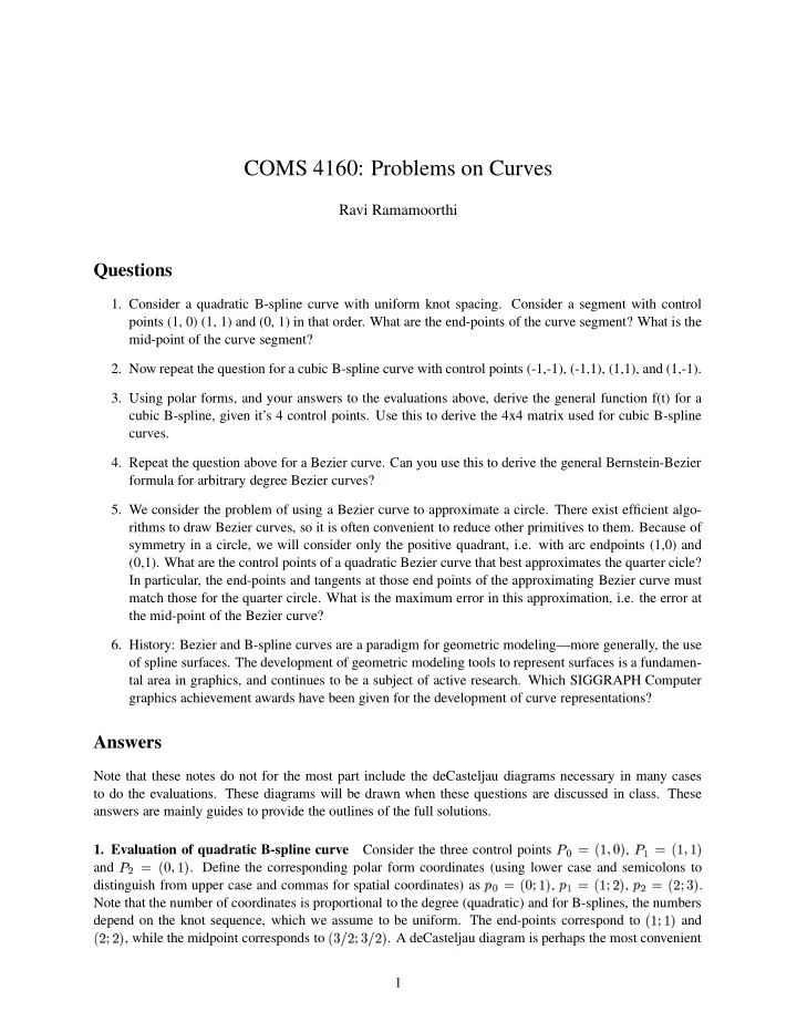
✛ ✛ ✛ COMS 4160: Problems on Curves Ravi Ramamoorthi Questions 1. Consider a quadratic B-spline curve with uniform knot spacing. Consider a segment with control points (1, 0) (1, 1) and (0, 1) in that order. What are the end-points of the curve segment? What is the mid-point of the curve segment? 2. Now repeat the question for a cubic B-spline curve with control points (-1,-1), (-1,1), (1,1), and (1,-1). 3. Using polar forms, and your answers to the evaluations above, derive the general function f(t) for a cubic B-spline, given it’s 4 control points. Use this to derive the 4x4 matrix used for cubic B-spline curves. 4. Repeat the question above for a Bezier curve. Can you use this to derive the general Bernstein-Bezier formula for arbitrary degree Bezier curves? 5. We consider the problem of using a Bezier curve to approximate a circle. There exist efficient algo- rithms to draw Bezier curves, so it is often convenient to reduce other primitives to them. Because of symmetry in a circle, we will consider only the positive quadrant, i.e. with arc endpoints (1,0) and (0,1). What are the control points of a quadratic Bezier curve that best approximates the quarter cicle? In particular, the end-points and tangents at those end points of the approximating Bezier curve must match those for the quarter circle. What is the maximum error in this approximation, i.e. the error at the mid-point of the Bezier curve? 6. History: Bezier and B-spline curves are a paradigm for geometric modeling—more generally, the use of spline surfaces. The development of geometric modeling tools to represent surfaces is a fundamen- tal area in graphics, and continues to be a subject of active research. Which SIGGRAPH Computer graphics achievement awards have been given for the development of curve representations? Answers Note that these notes do not for the most part include the deCasteljau diagrams necessary in many cases to do the evaluations. These diagrams will be drawn when these questions are discussed in class. These answers are mainly guides to provide the outlines of the full solutions. �✂✁☎✄✝✆✟✞✡✠☞☛✍✌ , �✏✎✑✄✒✆✟✞✡✠✓✞✔✌ 1. Evaluation of quadratic B-spline curve Consider the three control points �✖✕✗✄✘✆✙☛✚✠✓✞✔✌ . Define the corresponding polar form coordinates (using lower case and semicolons to and ✁✜✄✢✆✙☛✚✣✓✞✔✌ , ✎✤✄✥✆✟✞✡✣✧✦★✌ , ✕✩✄✪✆✫✦✬✣✧✭★✌ . distinguish from upper case and commas for spatial coordinates) as Note that the number of coordinates is proportional to the degree (quadratic) and for B-splines, the numbers ✆✟✞✡✣✓✞✔✌ and depend on the knot sequence, which we assume to be uniform. The end-points correspond to ✆✫✦✬✣✧✦★✌ , while the midpoint corresponds to ✆✫✭★✮✡✦✬✣✧✭★✮✡✦★✌ . A deCasteljau diagram is perhaps the most convenient 1
✭ � ✪ ✯ ✪ ✏ ✁ ✁ ✄ ✠ � ✁ ✎ ✄ ✄ ✕ � ✦ ✟ ✟ � ✎ ✌ ✄ ✕ � ✄ ✎ � ✟ ✟ ✠ ✭ ✟ ✦ ✄ � ✁ � ✎ ✄ ✁ ✦ ✕ � ✎ ✦ ✄ ✁ ✠ � ✯ � ✄ ✁ ✪ ✎ ✄ ✁ � ✏ ✎ ✄ � � ✯ � ✁ ✄ ✄ ✁ ✭ ✎ ✁ ✄ � ✟ ✁ ✠ ✠ ✄ ✪ ✌ ✭ ✮ ✞ ✄ ✎ ✁ ✪ � ✝ � ✞ ✞ ✆ ✎ ✕ ✠ ✖ ✁ ✁ ✄ � ✭ ✁ ✞ � ✞ � ✞ ✠ ✁ ✖ ✖ � � ✁ ✄ � ✎ � ✎ ✦ ✞ ✎ ✌ ✒ ✝ ✄ ✄ ✤ ☞ ✍ ✤ ✕ ✖ ✎ ✧ ✄ ✧ ✝ ✁ ✫ ✟ ✪ ✭ ✄ ✭ ✖ ✎ � ✁ ✄ � ✔ � ✁ ✭ ✖ ✝ � ✎ ✄ ✄ ✔ ✌ method for evaluation and will be shown in class. Here, we detail the main steps. We want to find the ✁ and ✎ and the final point on the curve. intermediate points ✆✟✞✡✣✓✞✔✌ and it corresponds directly to the ✁✤✄ First, let us consider the left endpoint. The polar form for final value sought. This is clearly given by ✁ ✄✂ ✞✡✠ ✄ ✆☎ (1) ✦ ✞✝✠✟ ✎✩✄✝✆✫✦✬✣✧✦★✌ and the value is ✎✩✄✝✆✙�✏✎ ✡✂ By symmetry, the right endpoint is given by the polar form for ✠✓✞✔✌ . ✕✔✌ ✮✡✦✑✄ ✆✟✞✡✣✧✭★✮✡✦★✌ and ✆✫✦✬✣✧✭★✮✡✦★✌ and then take Now, consider the midpoint. We need to use polar form the midpoint. In this case, ✞✡✠ ☛✌☞✎✍✑✏✎☛✓✒ ✄ ✕☎ ✠✓✞ ☛✘✗✙✍✑✏✎☛✓✒ ✄ ✕☎ ✚✜✛✣✢ ✄ ✕☎✦✥ ✠ ✓✥ (2) ✆✙☛✚✣✓✞✡✣✧✦★✌ ✆✟✞✡✣✧✦✬✣✧✭★✌ ✆✫✦✚✣✧✭✚✣ ✎✖ ✆✫✭✚✣ ✎✖ ✣ ✩★ ★✌ 2. Evaluation of cubic B-spline curve For the cubic curve, the polar forms are ✆✫✭✬✣✧✭✬✣✧✭★✌ and the midpoint ★ ★✌ . ✆✫✦✬✣✧✦✬✣✧✦★✌ ✆✫✦ ★ ✬✣✧✦ ★ ✬✣✧✦ with the desired end points being ✕ followed ✁✡✠ First, consider the left endpoint. We will be interested in the 3 intermediate values ✎ . For the left endpoint, we have polar forms ✁✡✠ by the 2 at the next step ✆✟✞✡✣✧✦✬✣✧✦★✌ ✆✫✦✬✣✧✦✬✣✧✭★✌ ✁✤✄ ✆✫✦✬✣✧✦✬✣✧✦★✌ ✠ ✎✫ (3) ✕ or ✫ ★✎ . Now, We don’t care about ✦✡�✏✎ ✬✂ �✖✁ ✦✡�✏✎ ✭✂ �✖✕ (4) and the final value �✖✁ ✄✂✮✖ ★� ✁ ✄✂ ✎ ✬✂ (5) ✯ . Evaluating these, we obtain that ✆✙�✏✎ ✰✂✱✖ ★�✖✕ ✡✂ Similar, for the right end-point, the final value ✦★✮✡✭✬✠✧✦★✮✡✭★✌ and ✆✫✦★✮✡✭✬✠✧✦★✮✡✭★✌ . ✆ ✙✲ the left and right endpoints are given respectively by Now, consider the midpoint. For these, we are interested in polar forms ✆✟✞✡✣✧✦✬✣ ✳★ ★✮✡✦★✌ ✆✫✦✬✣✧✭✬✣ ✳★ ★✮✡✦★✌ ✕✤✄ ✆✫✭✬✣ ✎✖ ✣ ✳★ ★✮✡✦★✌ (6) The corresponding points are given by �✖✁ ✄✂✴★ ✡�✏✎ �✏✎ ✬✂ �✖✕ ★ ✡�✖✕ ✄✂ (7) Evaluating these, we obtain, ✞✡✠ ✆✙☛✚✠✓✞✔✌ ✆✟✞✡✠ ✆ ✙✲ (8) ✆✫✭✬✣ ✳★ ★✮✡✦✬✣ ✳★ ★✮✡✦★✌ , and the values are ✆✫✦✬✣ ✳★ ★✮✡✦✬✣ ✳★ ★✮✡✦★✌ ✠ ✎✫ At the next level, the polar forms are ✁ ✰✂ ✕ ✄✂ ✄ ✆☎✵✲ ✄ ✶☎ (9) ✞✓✦ ✞✓✦ ✝✠✟ ✞✔✮✬✞✓✦★✌ . ✆✙☛✚✠✓✞ Finally, the value we seek, which is the midpoint of these, evaluates simply to 2
Recommend
More recommend
Explore More Topics
Stay informed with curated content and fresh updates.
