Computer Practical Exercise using GCTA (with PLINK and R) Overview - PDF document
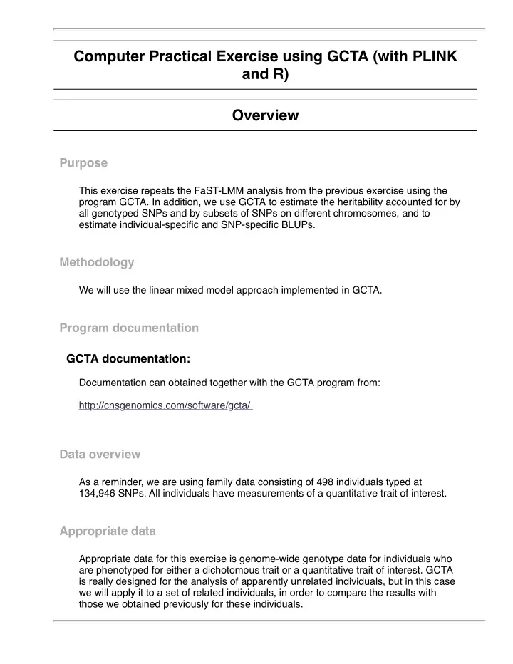
Computer Practical Exercise using GCTA (with PLINK and R) Overview Purpose This exercise repeats the FaST-LMM analysis from the previous exercise using the program GCTA. In addition, we use GCTA to estimate the heritability accounted for by
Computer Practical Exercise using GCTA (with PLINK and R) Overview Purpose This exercise repeats the FaST-LMM analysis from the previous exercise using the program GCTA. In addition, we use GCTA to estimate the heritability accounted for by all genotyped SNPs and by subsets of SNPs on different chromosomes, and to estimate individual-specific and SNP-specific BLUPs. Methodology We will use the linear mixed model approach implemented in GCTA. Program documentation GCTA documentation: Documentation can obtained together with the GCTA program from: http://cnsgenomics.com/software/gcta/ Data overview As a reminder, we are using family data consisting of 498 individuals typed at 134,946 SNPs. All individuals have measurements of a quantitative trait of interest. Appropriate data Appropriate data for this exercise is genome-wide genotype data for individuals who are phenotyped for either a dichotomous trait or a quantitative trait of interest. GCTA is really designed for the analysis of apparently unrelated individuals, but in this case we will apply it to a set of related individuals, in order to compare the results with those we obtained previously for these individuals.
Instructions Data files We will use the same PLINK binary-file format files quantfamdata.bed , quantfamdata.bim and quantfamdata.fam used previously. In addition, we will make use of a file topsnps.txt that lists the top SNPs on chromosomes 6 and 12 from our previous FaST-LMM analysis. We will also use R to create an additional phenotype file required by GCTA. Step-by-step instructions 1. Create new data files in PLINK and R To start with, we will use PLINK and R to create some additional data files that will be useful later on. First we will use PLINK to create a file that lists the genotypes (coded as 0,1,2) at the top SNPs from the FaST-LMM analysis. Type head FLMMresults more topsnps.txt to check that the file topsnps.txt does indeed list the top SNPs on chromosomes 6 and 12 from the FaST-LMM analysis. Run PLINK by typing: plink --bfile quantfamdata --extract topsnps.txt --recodeA --out topsnpsFLMM and take a look at the output file topsnpsFLMM.raw to check you understand how it is coded. Start R (by typing R ) and create a new phenotype file from the .fam file by typing the following commands: fam<-read.table("quantfamdata.fam", header=F) pheno=data.frame(fam[,1:2],fam[,6]) write.table(pheno,file="phenos.txt",col.names=F,row.names=F,quote=F) Take a look at the file phenos.txt that you created, to check you understand it. 2. GCTA Analysis To use GCTA to perform association analysis while allowing for relatedness between individuals, type: gcta64 --mlma --bfile quantfamdata --pheno phenos.txt --out GCTAresults
Here we use the --mlma option to tell GCTA to perform association analysis, we use the --bfile and --pheno options to tell GCTA which files to read in the genotype and phenotype data from, and we use GCTAresults as the stem name for the output files. To calculate the genomic control inflation factor, and to produce QQ and Manhattan plots from the above analysis, you can use the following sequence of commands within R. (Make sure that you understand the commands - if not please ask an instructor). source("qqmanHJCupdated.R") res3<-read.table("GCTAresults.mlma", header=T) head(res3) chi<-(qchisq(1-res3$p,1)) lambda=median(chi)/0.456 lambda new3<-data.frame(res3$SNP, res3$Chr, res3$bp, res3$p) names(new3)<-c("SNP", "CHR", "BP", "P") head(new3) qq(new3$P) manhattan(new3, pch=20, suggestiveline=F, genomewideline=F, ymin=2, cex.x.axis=0.65, colors=c("black","dodgerblue"), cex=0.5) You should find that the genomic control factor is close to 1.0, and the QQ and Manhattan plots are similar to those you obtained from FaST-LMM. To compare the results ( res3 ) with our previous FaST-LMM results ( res2 ), use the following sequence of commands within R: res2<-read.table("FLMMresults", header=T) new2<-data.frame(res2$SNP, res2$Chromosome, res2$Position, res2$Pvalue) names(new2)<-c("SNP", "CHR", "BP", "P") merged=merge(new3,new2, by="SNP", sort=F) head(res2) head(new2) head(new3) head(merged) plot(-log10(merged$P.x),-log10(merged$P.y)) abline(0,1) You should find that the GCTA results (on the x axis) are very similar to the FaST- LMM results (on the y axis), although the -log10 P-values from FaST-LMM are consistently just a little bit higher than those from GCTA. To use GCTA to estimate the heritability accounted for by all autosomal genome-wide SNPs, you need to first estimate the GRM, and then use the GRM to estimate the (SNP) heritability. This can be achieved using the following commands: gcta64 --bfile quantfamdata --autosome --make-grm-bin --out GCTAgrm gcta64 --reml --grm-bin GCTAgrm --pheno phenos.txt --out GCTAherit The screen output estimates the SNP heritability V(G)/Vp to be 0.480589 or around
48%. To estimate the heritabilty accounted for by SNPs on chromosomes 1, 2, 6 and 12 (for example), use the following commands: gcta64 --bfile quantfamdata --chr 1 --make-grm-bin --out GCTAgrmchr1 gcta64 --reml --grm-bin GCTAgrmchr1 --pheno phenos.txt --out GCTAheritchr1 gcta64 --bfile quantfamdata --chr 2 --make-grm-bin --out GCTAgrmchr2 gcta64 --reml --grm-bin GCTAgrmchr2 --pheno phenos.txt --out GCTAheritchr2 gcta64 --bfile quantfamdata --chr 6 --make-grm-bin --out GCTAgrmchr6 gcta64 --reml --grm-bin GCTAgrmchr6 --pheno phenos.txt --out GCTAheritchr6 gcta64 --bfile quantfamdata --chr 12 --make-grm-bin --out GCTAgrmchr12 gcta64 --reml --grm-bin GCTAgrmchr12 --pheno phenos.txt --out GCTAheritchr12 You should find that the SNP heritabilities on chromosomes 1 and 2 do not look particularly significant (given the estimated standard errors), but the SNP heritabilities on chromosomes 6 and 12 are significant (as might be expected from the strong effects seen on these chromosomes). The sum of the SNP heritabilities on these 4 chromosomes (0.20647+0.111512+0.368184+0.286570) adds up to more then the overall SNP heritability of 0.480589. This is due to the phenomenon that, in the presence of population substructure or close relatedness, chromosome-specific heritability estimates can be confounded by shared non-genetic effects (for examples shared environment) or corrrelations between SNPs on different chromosomes, leading to an over-estimate of the chromosome-specific heritability. To correctly partition the overall heritability between the 22 autosomes, we need to first estimate chromosome-specific GRMs and then include them all simultaneously in the model: gcta64 --bfile quantfamdata --chr 1 --make-grm-bin --out GCTAgrmchr1 gcta64 --bfile quantfamdata --chr 2 --make-grm-bin --out GCTAgrmchr2 gcta64 --bfile quantfamdata --chr 3 --make-grm-bin --out GCTAgrmchr3 gcta64 --bfile quantfamdata --chr 4 --make-grm-bin --out GCTAgrmchr4 gcta64 --bfile quantfamdata --chr 5 --make-grm-bin --out GCTAgrmchr5 gcta64 --bfile quantfamdata --chr 6 --make-grm-bin --out GCTAgrmchr6 gcta64 --bfile quantfamdata --chr 7 --make-grm-bin --out GCTAgrmchr7 gcta64 --bfile quantfamdata --chr 8 --make-grm-bin --out GCTAgrmchr8 gcta64 --bfile quantfamdata --chr 9 --make-grm-bin --out GCTAgrmchr9 gcta64 --bfile quantfamdata --chr 10 --make-grm-bin --out GCTAgrmchr10 gcta64 --bfile quantfamdata --chr 11 --make-grm-bin --out GCTAgrmchr11 gcta64 --bfile quantfamdata --chr 12 --make-grm-bin --out GCTAgrmchr12 gcta64 --bfile quantfamdata --chr 13 --make-grm-bin --out GCTAgrmchr13 gcta64 --bfile quantfamdata --chr 14 --make-grm-bin --out GCTAgrmchr14 gcta64 --bfile quantfamdata --chr 15 --make-grm-bin --out GCTAgrmchr15 gcta64 --bfile quantfamdata --chr 16 --make-grm-bin --out GCTAgrmchr16 gcta64 --bfile quantfamdata --chr 17 --make-grm-bin --out GCTAgrmchr17 gcta64 --bfile quantfamdata --chr 18 --make-grm-bin --out GCTAgrmchr18 gcta64 --bfile quantfamdata --chr 19 --make-grm-bin --out GCTAgrmchr19 gcta64 --bfile quantfamdata --chr 20 --make-grm-bin --out GCTAgrmchr20 gcta64 --bfile quantfamdata --chr 21 --make-grm-bin --out GCTAgrmchr21 gcta64 --bfile quantfamdata --chr 22 --make-grm-bin --out GCTAgrmchr22 gcta64 --reml --mgrm-bin multipleGRMs.txt --pheno phenos.txt --out GCTAherit22GRMs
Recommend
More recommend
Explore More Topics
Stay informed with curated content and fresh updates.
