Computer Graphics and GPGPU Programming Donato DAmbrosio Department - PowerPoint PPT Presentation
Computer Graphics and GPGPU Programming Donato DAmbrosio Department of Mathematics and Computer Science and Center of Excellence for High Performace Computing Cubo 22B, University of Calabria, Rende 87036, Italy mailto:
Computer Graphics and GPGPU Programming Donato D’Ambrosio Department of Mathematics and Computer Science and Center of Excellence for High Performace Computing Cubo 22B, University of Calabria, Rende 87036, Italy mailto: donato.dambrosio@unical.it homepage: http://www.mat.unical.it/~donato Academic Year 2018/19 Donato D’Ambrosio (University of Calabria) Academic Year 2018/19 1 / 51
Algorithms Table of contents Algorithms 1 Clipping Rasterization Hidden surface removal Light 2 The Phong Model Shading Donato D’Ambrosio (University of Calabria) Academic Year 2018/19 2 / 51
Algorithms Algorithms Algorithms Donato D’Ambrosio (University of Calabria) Academic Year 2018/19 3 / 51
Algorithms Stages of the OpenGL ’s Graphics Process The graphics process can be split in the following stages: Modeling (the 3D scene is conceptually defined by means of vertices in a vectorial context) Vertex Processing Primitives (e.g. triangles) are defined Primitives laying outside the clip space are discarded (clipping) Hidden primitives are discarded (hidden surface removal) Rasterization The scene is converted into a raster image (image’s elements are called fragments) Fragment processing (a color is assigned to each fragment) Output merging (combine the fragments of all primitives into color pixels for the display) Donato D’Ambrosio (University of Calabria) Academic Year 2018/19 4 / 51
Algorithms Clipping Clipping Clipping is the process that discards (entirely or partially) the primitives that are outside the clip space The primitives within the clip space are accepted, while the other are eliminated or rejected The primitives that are partially within the clip space are cut and new vertices added in order to obtain a new primitive that is entirely within the clip space Donato D’Ambrosio (University of Calabria) Academic Year 2018/19 5 / 51
Algorithms Clipping Clipping Evaluating the intersections with the clip planes is the most important computational effort in clipping algorithm Accordingly, it is important to minimize the number of intersections (since they require floating point operations) Donato D’Ambrosio (University of Calabria) Academic Year 2018/19 6 / 51
Algorithms Clipping Cohen-Sutherland’s clipping algorithm Let consider the two-dimensional case (it is conceptually equivalent to the three-dimensional one) The edges of the clipping plane are ideally extended to the infinitive by forming 9 regions A 4 bit code O = b 0 b 1 b 2 b 3 , called outcode, is assigned to each region Donato D’Ambrosio (University of Calabria) Academic Year 2018/19 7 / 51
Algorithms Clipping Cohen-Sutherland’s clipping algorithm Outcodes are defined by the following rule: � 1 if y > y max b 0 = 0 if y ≤ y max Similarly, b 1 = 1 if y < y min b 2 and b 3 are defined by relations between x and the left and right edges of the clip region Note that the clip region has outcode O = 0000 Donato D’Ambrosio (University of Calabria) Academic Year 2018/19 8 / 51
Algorithms Clipping Cohen-Sutherland’s clipping algorithm Case 1: O 1 = O 2 = 0000 Both outcode are 0000. The segment is INTERNAL Case 2: O 1 & O 2 � = 0000 The extremes are both up, down, to the left or to the right of the clip window. The segment is EXTERNAL Case 3: O 1 & O 2 = 0000 The extremes are external but the line can not be rejected since it could intersect the window. Intersections with the clip window’s edges must be computed and if the line actually intersects the clip region new vertces evaluated Case 4: O 1 � = 0000 ; O 2 = 0000, or viceversa The line is partially outside the clip window. In this case, the vertex outside the window is replaced by a ne vertex resulting from the intersection between the line and the clip window’s edge Donato D’Ambrosio (University of Calabria) Academic Year 2018/19 9 / 51
Algorithms Rasterization Scan conversion of segments Starting from the vertices of the primitive projected into the two-dimensional plane, the rasterization or scan conversion builds the primitive as a set of fragments Let us suppose the vertices composing the geometric primitives have already been projected on a n × m matrix with the origin located at the bottom-left pixel Let us suppose that each pixel is a square with the center at the pixel coordinates and side equal to the distance between two adjacent pixels Donato D’Ambrosio (University of Calabria) Academic Year 2018/19 10 / 51
Algorithms Rasterization The DDA line algorithm Let us suppose to have a segment defined by its extremes ( x 1 , y 1 ) and ( x 2 , y 2 ) The slope of the segment is defined as: m = ∆ y / ∆ x The most simple scan conversion algorithm evaluates m , increments x (starting from the left extreme), and computes y i = mx i + h , where h is the ordinata of the intersection between the y axis and the line, for each x i Donato D’Ambrosio (University of Calabria) Academic Year 2018/19 11 / 51
Algorithms Rasterization The DDA line algorithm The above strategy is inefficient since each iteration requires one floating point multiplication and one floating point addition It is possible to avoid the multiplication by adopting an incremental strategy so that one pixel can be computed based on the previous one This algorithm is called DDA 1 Each time x is incremented of ∆ x , the corresponding variation of y must be ∆ y = m ∆ x Ranging form x 1 to x 2 , x is incremented by 1 (i.e. the distance between two pixels) and then y is incremented by ∆ y = m 1 The name comes from the Digital Differential Analyzer, a mechanical device able to solve differential equations by applying a numerical methods Donato D’Ambrosio (University of Calabria) Academic Year 2018/19 12 / 51
Algorithms Rasterization The DDA line algorithm Let us assume that 0 ≤ m ≤ 1 (the other values can be treated equivalently) int x ; float dy , dx , y , m; dy = y2 − y1 ; dx = x2 − x1 ; m = dy / dx ; y = y1 ; for ( x = x1 , x <= x2 , x++) { w r i t e P i x e l ( x , round ( y ) , l i n e _ c o l o r ) ; y += m; } Donato D’Ambrosio (University of Calabria) Academic Year 2018/19 13 / 51
Algorithms Rasterization Bresenham’s line algorithm The DDA line algorithm is straightforward and easy to implement but execs a floating point operation for each line’s pixel At the contrary, the Bresenham’s line algorithm only performs integer operations Bresenham’s algorithm is faster than DDA and, for this reason, it has become the most used line algorithm in Computer Graphics *** Let us suppose to have a segment defined by its extremes ( x 1 , y 1 ) and ( x 2 , y 2 ) Donato D’Ambrosio (University of Calabria) Academic Year 2018/19 14 / 51
Algorithms Rasterization Bresenham’s line algorithm Let us suppose we are at an intermediate step of the algorithm and the pixel ( i , j ) was the last to be switched on As a consequence, when x = i the line y = mx + h intersects the pixel ( i , j ) When x = i + 1, the condition 0 ≤ m ≤ 1 implies that only one of the pixels ( i + 1 , j ) and ( i + 1 , j + 1 ) can be switched on The choice can be expressed by means of a decision variable d = b − a where a and b are the measures of lines starting from the centers of pixels ( i + 1 , j + 1 ) and ( i + 1 , j ) , respectively (as shown in the next figure), to the line y = mx + h and parallel to the y axis Donato D’Ambrosio (University of Calabria) Academic Year 2018/19 15 / 51
Algorithms Rasterization Bresenham’s line algorithm Definition of the decision variable d = b − a If d > 0 then the line y = mx + h is closest to the pixel ( i + 1 , j + 1 ) If d ≤ 0 then the line y = mx + h is closest to the pixel ( i + 1 , j ) d can be computed without the need of floating point operations by means of a recurrence formula where d i + 1 is a function of d i Donato D’Ambrosio (University of Calabria) Academic Year 2018/19 16 / 51
Algorithms Rasterization Bresenham’s line algorithm Case d i > 0 1 + b i + 1 = b i + m ⇒ b i + 1 = b i + m − 1 a i + 1 = 1 − b i + 1 = 1 − ( b i + m − 1 ) = 1 − ( 1 − a i + m − 1 ) = a i − m + 1 d i + 1 = b i + 1 − a i + 1 = b i − a i + 2 m − 2 = d i + 2 m − 2 = d i + 2 ( m − 1 ) Donato D’Ambrosio (University of Calabria) Academic Year 2018/19 17 / 51
Algorithms Rasterization Bresenham’s line algorithm Case d i ≤ 0 b i + 1 = b i + m a i + 1 = a i − m d i + 1 = b i + 1 − a i + 1 = b i − a i + 2 m = d i + 2 m Donato D’Ambrosio (University of Calabria) Academic Year 2018/19 18 / 51
Algorithms Rasterization Bresenham’s line algorithm So, we have � d i + 2 ( m − 1 ) if d > 0 d i + 1 = d i + 2 m if d ≤ 0 Since we are interested in the sign of d , we can multiply by ∆ x = x 2 − x 1 (that is a positive quantity) � d i ∆ x + 2 ( m − 1 )∆ x = d i ∆ x + 2 (∆ y − ∆ x ) if d > 0 d i + 1 ∆ x = d i ∆ x + 2 m ∆ x = d i ∆ x + 2 ∆ y if d ≤ 0 Eventually, we can impose d i = d i ∆ x (since both of them have the same sign) � 2 (∆ y − ∆ x ) if d > 0 d i + 1 = d i + 2 ∆ y if d ≤ 0 Donato D’Ambrosio (University of Calabria) Academic Year 2018/19 19 / 51
Recommend
More recommend
Explore More Topics
Stay informed with curated content and fresh updates.


