Computational Logic A Hands-on Introduction to Logic Programming 1 - PDF document

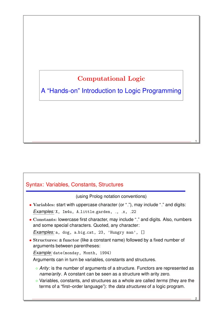
Computational Logic A “Hands-on” Introduction to Logic Programming 1 Syntax: Variables, Constants, Structures (using Prolog notation conventions) • Variables: start with uppercase character (or “ ”), may include “ ” and digits: Examples: X, Im4u, A little garden, , x, 22 • Constants: lowercase first character, may include “ ” and digits. Also, numbers and some special characters. Quoted, any character: Examples: a, dog, a big cat, 23, ’Hungry man’, [] • Structures: a functor (like a constant name) followed by a fixed number of arguments between parentheses: Example: date(monday, Month, 1994) Arguments can in turn be variables, constants and structures. ⋄ Arity: is the number of arguments of a structure. Functors are represented as name/arity . A constant can be seen as a structure with arity zero. ⋄ Variables, constants, and structures as a whole are called terms (they are the terms of a “first–order language”): the data structures of a logic program. 2

Syntax: Terms (using Prolog notation conventions) • Examples of terms : Term Type Main functor: dad constant dad/0 time(min, sec) structure time/2 pair(Calvin, tiger(Hobbes)) structure pair/2 Tee(Alf, rob) illegal — A good time variable — • Functors can be defined as prefix , postfix , or infix operators (just syntax!): is the term if +/2 declared infix a + b ’+’(a,b) is the term if -/1 declared prefix - b ’-’(b) a < b is the term ’<’(a,b) if </2 declared infix john father mary is the term father(john,mary) if father/2 declared infix We assume that some such operator definitions are always preloaded. 3 Syntax: Atoms, Literals • Atoms: an expression of the form: p( t 1 , t 2 , ..., t n ) ⋄ p is the atom’s predicate symbol (same convention as with functors), ⋄ n is its arity, ⋄ and t 1 , t 2 , ..., t n are terms . ⋄ The predicate symbol of an atom is also represented as p/n . • Atoms and terms are syntactically identical! They are distinguished by context: if dog(name(barry), color(black)) is an atom then name(barry) and color(black) are terms if color(dog(barry,black)) is an atom then dog(barry,black) is a term • I.e., atoms cannot appear inside terms; terms are the arguments of atoms. • Literals: A literal is a positive (non negated) or negative (negated) atom. 4

Syntax: Rules • Rules: A rule is an expression of the form: p 0 ( t 1 , t 2 , . . . , t n 0 ) ← p 1 ( t 1 1 , t 1 2 , . . . , t 1 n 1 ) , . . . p m ( t m 1 , t m 2 , . . . , t m n m ) . ⋄ The expression to the left of the arrow has to be an atom (no negation) and is called the head of the rule. ⋄ Those to the right of the arrow are literals and form the body of the rule. ⋄ Literals in the body of a rule are also called procedure calls . Example : meal(First, Second, Third) <- appetizer(First), main_dish(Second), dessert(Third). 5 Syntax: Facts, Clauses, Predicates • Facts: A fact is an expression of the form: p( t 1 , t 2 , ..., t n ) <-. (i.e., a fact is a rule with an empty body). Examples : dog(name(barry), color(black)) <-. friends(’Ann’, ’John’) <-. • Rules and facts are both called clauses . • Predicates: all clauses whose heads have the same name and arity form a predicate (or procedure ) definition. Example : pet(spot) <-. pet(X) <- animal(X), barks(X). pet(X) <- animal(X), meows(X). Predicate pet/1 has three clauses. Of those, one is a fact and two are rules. 6

Declarative Meaning of Facts and Rules The declarative meaning is the corresponding one in first order logic, according to certain conventions: • Rules: ⋄ Commas in rule bodies represent conjunction, i.e., p ← p 1 , · · · , p m . represents p ← p 1 ∧ · · · ∧ p m . ⋄ “ ← ” represents as usual logical implication. Thus, a rule p ← p 1 , · · · , p m . means “if p 1 and . . . and p m are true, then p is true” Example : the rule pet(X) <- animal(X), barks(X). can be read as “X is a pet if it is an animal and it barks”. • Facts : state things that are true. (Note that a fact p can be seen as the rule “ p <- true. ”) Example : the fact animal(spot) <-. can be read as “spot is an animal”. 7 Declarative Meaning of Predicates • Predicates : clauses in the same predicate p ← p 1 , ..., p n p ← q 1 , ..., q m ... provide different alternatives (for p ). Example : the rules pet(X) <- animal(X), barks(X). pet(X) <- animal(X), meows(X). express two ways for X to be a pet. • Note (variable scope ): the X variables in the two clauses above are different, even if they have the same name. Variables are local to clauses (and are renamed any time a clause is used). 8

Programs, Queries, and Execution • Logic Program: a set of predicates. Example : pet(X) <- animal(X), barks(X). pet(X) <- animal(X), meows(X). animal(spot) <-. barks(spot) <-. animal(barry) <-. meows(barry) <-. animal(hobbes) <-. roars(hobbes) <-. • Query: an expression of the form: ← p 1 ( t 1 1 , . . . , t 1 n 1 ) , . . . , p n ( t n 1 , . . . , t n n m ) . (i.e., a clause without a head). A query represents a question to the program . Example : <- pet(X). • Execution: given a program and a query, executing the logic programming is attempting to find an answer to the query . Example : above, the system will try to find a “substitution” for X which makes pet(X) true. Intuitively, we have two possible answers: spot and barry . The declarative semantics does not specify how this is done – this is the role of the operational semantics. 9 Operational Meaning • A logic program also has an operational meaning [Kowalski]: ⋄ A clause p ← p 1 ,...,p m . expresses: “to obtain (prove) p you have to obtain (prove) p 1 and ...and p m first” In principle, the order in which body literals p 1 , ..., p n are solved does not matter, but, for a given system this may be fixed. ⋄ A set of clauses: p ← p 1 , ..., p n p ← q 1 , ..., q m ... expresses “to prove p , prove p 1 ∧ ... ∧ p n , or prove q 1 ∧ ... ∧ q n , or . . . ” The presence of several applicable clauses for a given body literal means that several possible paths exist to a solution and they should be explored. Again, in principle, the order in which these paths are explored does not matter (if certain conditions are met), but, for a given system, this may also be fixed. 10

Unifi cation • Unifying two terms is finding (the minimal) values for the variables in those terms which make them syntactically equal. • Only variables can be given values! • Two terms can be made identical only by making identical their arguments. Example : Unify A With B Using θ ∅ dog dog { X = Y } X Y { X = a } X a f(X, g(t)) f(m(h), g(M)) { X = m(h) , M = t } Impossible (1) f(X, g(t)) f(m(h), t(M)) Impossible (2) f(X, X) f(Y, l(Y)) • (1) Terms with different name and/or arity cannot be unified. • (2) A variable cannot be given as value a term which contains that variable, because it would create an infinite term. This is known as the occurs check . • All applies to unification of atoms as well! 11 Substitutions • If the equation A = B has a solution then A and B are unifiable . • Solutions of a set of term equations are called substitutions . • In a solution all values for the variables are completely explicit! • Substitution: a set of equations assigning values to variables, with: ⋄ Only variables on the left hand side of each equation. ⋄ Only one equation for each left hand side variable. ⋄ Variables on the left hand side cannot appear on the right of any equation. Example : Set of Equations Substitution { X = f(Y) , Y = f(Z) } NO { X = f(f(Z)) , Y = f(Z) } YES { X = f(f(Z)) , Z = Y } NO { X = f(f(Z)) , Y = Z } YES { X = l(Y) , Y = l(Y) } NO (2) { X = l(Y) , X = Y } NO! 12

Unifi ers • A substitution θ which is a solution of A = B is called a unifier of A and B . • Most general unifier: one which assigns to the variables the values strictly required to unify. • Given two terms, if they are unifiable, then there exists a unique (up to variable renaming) most general unifier (m.g.u.) for them. Example : Unifiers MGU (unique!) Terms { X = m(a) , H = a , M = b , T = b } { X = m(H) , M = T } f(X, g(T)) f(m(H), g(M)) { X = m(H) , M = f(A) , T = f(A) } { X = m(A) , H = A , M = B , T = B } • Unifying two terms: find the minimal substitution which makes them identical. • Unification should find the (unique) m.g.u., if it exists, or fail otherwise. 13 Unifi cation Algorithm • Let A and B be two terms: 1 θ = ∅ , E = { A = B } 2 while not E = ∅ : 2.1 delete an equation T = S from E 2.2 case T or S (or both) are (distinct) variables. Assuming T variable: * (occur check) if T occurs in the term S → halt with failure * substitute variable T by term S in all terms in θ * substitute variable T by term S in all terms in E * add T = S to θ 2.3 case T and S are non-variable terms: * if their names or arities are different → halt with failure * obtain the arguments { T 1 , . . . , T n } of T and { S 1 , . . . , S n } of S * add { T 1 = S 1 , . . . , T n = S n } to E 3 halt with θ being the m.g.u of A and B 14