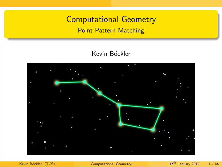
Computational Geometry Point Pattern Matching Kevin B ockler - PowerPoint PPT Presentation

Computational Geometry Point Pattern Matching Kevin B¨ ockler Institut f¨ ur Theoretische Informatik Universit¨ at zu L¨ ubeck 17 th January 2012 17 th January 2012 Kevin B¨ ockler (TCS) Computational Geometry 1 / 44

Topics Introduction 1 Matching of Point Patterns 2 Matching of Curves & Areas 3 Shape Interpolation 4 17 th January 2012 Kevin B¨ ockler (TCS) Computational Geometry 2 / 44

Introduction Introduction 1 Motivation Hausdorff-Distance Matching of Point Patterns 2 Exact Matching Approximated Matching Pattern recognition Matching of Curves & Areas 3 Approximated Matching Better distance for shapes Shape Interpolation 4 Polygonal chain matching Difficulties 17 th January 2012 Kevin B¨ ockler (TCS) Computational Geometry 3 / 44

Introduction Motivation Applications Distance of two shapes or: How similar is one shape compared to another? Applications: Computer vision/computations Molecular biology Sign recognition Morphing 17 th January 2012 Kevin B¨ ockler (TCS) Computational Geometry 4 / 44

Introduction Motivation The Problem Input: two shapes (set of points), P, Q ⊂ R 2 allowed transformations T of P, Q Output: f ∈ T , which solves one of the following problems: Exact matching Approximated matching Optimal matching 17 th January 2012 Kevin B¨ ockler (TCS) Computational Geometry 5 / 44

Introduction Motivation Transformations We define a transformation as follows: Transformation A transformation f is a function which maps one shape to another: Let A be a shape, e.g. a set of points: A = { a ∈ R 2 | a ∈ A } f : R 2 → R 2 Applying f on a shape means transforming of each element by f : f ( A ) = { f ( a ) | a ∈ A } 17 th January 2012 Kevin B¨ ockler (TCS) Computational Geometry 6 / 44

Introduction Motivation Transformations We look at the following transformations: Translation by t Rotation by ϑ Scaling by a Combinations Rigid Motion means translation and rotation Similarity means translation, rotation and scaling Rigid Motions are interesting! 17 th January 2012 Kevin B¨ ockler (TCS) Computational Geometry 7 / 44

Introduction Hausdorff-Distance Hausdorff-Distance What is the distance between two shapes? How similar are two shapes? 17 th January 2012 Kevin B¨ ockler (TCS) Computational Geometry 8 / 44

Introduction Hausdorff-Distance Hausdorff-Distance Definition The Hausdorff-Distance is the maximum of the minimal distances: δ H ( P, Q ) = max p ∈ P min q ∈ Q || p − q || 2 17 th January 2012 Kevin B¨ ockler (TCS) Computational Geometry 9 / 44

Introduction Hausdorff-Distance Overview of the problems Input: P, Q ⊂ R 2 and T of P, Q Output: f ∈ T with property of matching: Exact matching δ H ( f ( P ) , Q ) = 0 Approximated matching with ε as allowed error tolerance δ H ( f ( P ) , Q ) ≤ ε Optimal matching δ H ( f ( P ) , Q ) = min f ′ ∈ T δ H ( f ′ ( P ) , Q ) 17 th January 2012 Kevin B¨ ockler (TCS) Computational Geometry 10 / 44

Matching of Point Patterns Introduction 1 Motivation Hausdorff-Distance Matching of Point Patterns 2 Exact Matching Approximated Matching Pattern recognition Matching of Curves & Areas 3 Approximated Matching Better distance for shapes Shape Interpolation 4 Polygonal chain matching Difficulties 17 th January 2012 Kevin B¨ ockler (TCS) Computational Geometry 11 / 44

Matching of Point Patterns Exact Matching Exact matching Definition An exact matching of two sets P, Q is a valid function which transforms each point p ∈ P to a point q ∈ Q . or: δ H ( f ( P ) , Q ) = 0 Given: sets P, Q and T = T translations Output: f ( x ) ∈ T translations Exact matching means a translated point is equal to a point of q: ∀ p ∈ P : p ′ = f ( p ) = q, q ∈ Q 17 th January 2012 Kevin B¨ ockler (TCS) Computational Geometry 12 / 44

Matching of Point Patterns Exact Matching A simple algorithm for rigid motions 1 Compute the centroids c P , c Q 2 Sort all points of P, Q as pairs of (Φ i , r i ) and put them into a sequence 3 A matching is found, if the sorted sequence of P is a cyclic shift of the sequence of Q 4 If there is a matching, just compute the transformation by looking at the first pair of each P, Q Runtime: O ( n log( n )) 17 th January 2012 Kevin B¨ ockler (TCS) Computational Geometry 13 / 44

Matching of Point Patterns Exact Matching Extend with Scaling Considering Scaling is simple: Start the algorithm by finding a scaling factor Compute the diameters of P, Q 1 The scaling factor a is d P 2 d Q Computing scaling needs additional linear time 17 th January 2012 Kevin B¨ ockler (TCS) Computational Geometry 14 / 44

Matching of Point Patterns Approximated Matching Exact matching does not work! Exact matching � = Reality Approximation is more effective Problem: Approximated Matching Approximated matching means matching all points p ∈ P to the ε - neighborhood of a point q ∈ Q . one-to-one matching many-to-one matching For a given P, Q, T, ε : is there a matching? For a given P, Q, T : find the smallest ε 17 th January 2012 Kevin B¨ ockler (TCS) Computational Geometry 15 / 44

Matching of Point Patterns Approximated Matching One-to-one Matching: Approaching under rigid motions Given: sets A, B and T = T rigid motions Output: Is there a matching f ∈ T so, that B is matched to A within ε ? For each pair ( b i , b j ) find an interval of degree Φ All relationships are edges in a bipartite graph A matching does exist, if there is a perfect matching in this graph 17 th January 2012 Kevin B¨ ockler (TCS) Computational Geometry 16 / 44

Matching of Point Patterns Approximated Matching One-to-one Matching: Approaching under rigid motions Runtime of this approach: 1 Procedure has to be done n 4 times for all 4-tuples 2 For each procedure look at all 2-tuples’ curves and calculate intervals ⇒ Analysis showed runtime: O ( n 8 ) Other approaches: Translation only in O ( n 1 . 5 log( n )) Disjoint ε -neighborhoods lead to O ( n 4 log ( n )) + Assuming, ε is not too close at optimal ε min : O ( n 2 log ( n )) 17 th January 2012 Kevin B¨ ockler (TCS) Computational Geometry 17 / 44

Matching of Point Patterns Approximated Matching Many-to-One Matching: Hausdorff-Distance Matching by minimizing the Hausdorff-Distance Input: Sets P, Q with m = | P | , n = | Q | Many-to-One Matching Hausdorff-Distance computation in O ( mn ) by computing straight forward O ( m + n log( m + n )) by using Voronoi-Diagrams General idea: Take a transformation 1 Compute the new Hausdorff-Distance 2 Compare the result and repeat until a good transformation has been 3 found 17 th January 2012 Kevin B¨ ockler (TCS) Computational Geometry 18 / 44

Matching of Point Patterns Approximated Matching Many-to-One Matching: Goodrich approximation 1 For one diametrically opposing pair of points p 1 , p 2 ∈ P : 2 Do a best match to each pair of points q 1 , q 2 ∈ Q 3 Take the matching with the best resulting Hausdorff-distance T min = min T δ h ( T ( P ) , Q ) 17 th January 2012 Kevin B¨ ockler (TCS) Computational Geometry 19 / 44

Matching of Point Patterns Approximated Matching Many-to-One Matching: Goodrich approximation 1 For one diametrically opposing pair of points p 1 , p 2 ∈ P : 17 th January 2012 Kevin B¨ ockler (TCS) Computational Geometry 19 / 44

Matching of Point Patterns Approximated Matching Many-to-One Matching: Goodrich approximation 1 For one diametrically opposing pair of points p 1 , p 2 ∈ P : 2 Do a best match to each pair of points q 1 , q 2 ∈ Q 17 th January 2012 Kevin B¨ ockler (TCS) Computational Geometry 19 / 44

Matching of Point Patterns Approximated Matching Many-to-One Matching: Goodrich approximation 1 For one diametrically opposing pair of points p 1 , p 2 ∈ P : 2 Do a best match to each pair of points q 1 , q 2 ∈ Q 3 Take the matching with the best resulting Hausdorff-distance T min = min T δ h ( T ( P ) , Q ) 17 th January 2012 Kevin B¨ ockler (TCS) Computational Geometry 19 / 44

Matching of Point Patterns Approximated Matching Many-to-One Matching: Goodrich approximation 1 For one diametrically opposing pair of points p 1 , p 2 ∈ P : 2 Do a best match to each pair of points q 1 , q 2 ∈ Q 3 Take the matching with the best resulting Hausdorff-distance T min = min T δ h ( T ( P ) , Q ) 17 th January 2012 Kevin B¨ ockler (TCS) Computational Geometry 19 / 44

Matching of Point Patterns Approximated Matching Many-to-One Matching: Goodrich approximation 1 For one diametrically opposing pair of points p 1 , p 2 ∈ P : 2 Do a best match to each pair of points q 1 , q 2 ∈ Q 3 Take the matching with the best resulting Hausdorff-distance Runtime of the Goodrich approximation: m = | P | , n = | Q | 1 O ( m ) 2 O ( n 2 ) 3 O ( n 2 m log( n )) Runtime is O ( n 2 m log( n )) 17 th January 2012 Kevin B¨ ockler (TCS) Computational Geometry 20 / 44

Matching of Point Patterns Pattern recognition Alignment Method Given a model M and a scene S : Does S contain M ? Reference Frame A reference frame of a set M in dependency of two offset points a, b ∈ M represents a new coordinate system with properties: a is assigned as the origin (0 , 0) b is assigned as an alignment vector (1 , 0) all other points relate to these two points 17 th January 2012 Kevin B¨ ockler (TCS) Computational Geometry 21 / 44