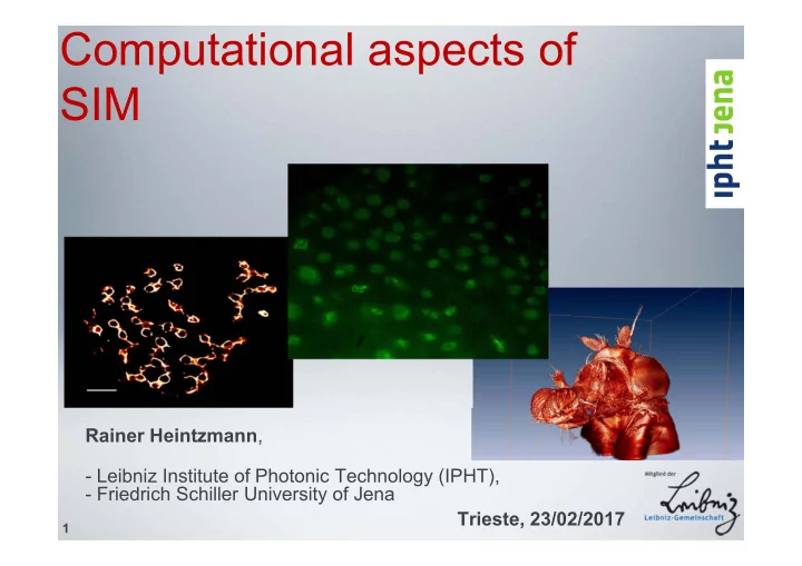
Computational aspects of SIM Rainer Heintzmann , - Leibniz - PowerPoint PPT Presentation
Computational aspects of SIM Rainer Heintzmann , - Leibniz Institute of Photonic Technology (IPHT), - Friedrich Schiller University of Jena Trieste, 23/02/2017 1 Paradigm: Optimize for direct visibility + Image Object Optics E.g.:
Computational aspects of SIM Rainer Heintzmann , - Leibniz Institute of Photonic Technology (IPHT), - Friedrich Schiller University of Jena Trieste, 23/02/2017 1
Paradigm: Optimize for direct visibility � + Image Object Optics E.g.: Widefield, Confocal, STED Does not necessarily optimize information content!
Paradigm: Optimize for information content � + Object Optics Data Data Image Computation � +
Examples in Medical Imaging MRI SPECT http://www.cis.rit.edu/htbooks/mri/images/head.gif http://www.physics.ubc.ca/research/images/spect.gif PET fMRI CT http://www.cerebromente.org.br/n01/pet/petdep.gif http://www.fmri.wfubmc.edu/other%20pics/ http://www.vetmed.lsu.edu/vth&c/Orthopedics/Images/ lab_brain_logo.JPG Computed%20Tomography%20(CT)%20Scanner.RV.jpg
Structured Illumination (SIM) 5
Moiré Demonstration
7 Moiré effect high frequency ... is lost detail Sample Aurélie Jost Aurélie Jost
Moiré effect 8 high frequency Illumination grid HF information is present high frequency low frequency Sample Moiré detail Aurélie Jost Aurélie Jost
The Moiré effect Moiré fringes Image: Wikipedia (author:Ildar Sagdejev)
Image formation in FLUORESCENCE I em ( x ) = Obj( x ) · I ex ( x ) Multiplication in real space ↕ Convolution in Fourier space ~ ~ ~ I em ( k ) = Obj( k ) � I ex ( k )
Object Fluorescence Distribution I em ( x ) = Obj( x ) · I ex ( x ) ~ ~ ~ I em ( k ) = Obj( k ) � I ex ( k ) detectable region magnitude ~ I em ( k ) ~ � 0 Image ( k ) - � 0 ~ Obj + 1 (k) -K 0 +K spatial freq.
Piecing Parts Together • Correct for OTF • Extract components • Shift into place • Weighted average • Apodize detectable region magnitude ~ I em ( k ) ~ � 0 Image ( k ) - � 0 ~ Obj + 1 (k) -K 0 +K spatial freq.
Structured Illumination Micropscopy Sample Sample with structured illumination Illumination Multiplication of sample and illumination
Structured Illumination Micropscopy Sample Illumination
Structured Illumination Micropscopy Sample
Structured Illumination Micropscopy Sample Sample & llumination
Sample Sample & llumination Imaging leads to loss of high frequencies (OTF)
Sample Separating the components…
Sample Separating the components… Shifting the components…
Sample Separating the components… Shifting the components… Recombining the components…
Sample Reconstructed sample Separating the components… Shifting the components… Recombining the components … using the correct weights. Image processing !
Multiple images for order separation CCD x z Tube lens Tube lens Filter Dichromatic Laser reflector Diffraction grating, SLM, etc… Objective Sample
3D Structured Illumination Microtubule cytoskeleton in HeLa cells M.G.L Gustafsson et al ., Three-dimensional Resolution Doubling in Widefield Fluorescence Microscopy by Structured Illumination, Biophys. J. (BioFAST), 2008
Microscopy image Resolution map shifted information shifted information shifted information shifted information Reconstruct high resolution image like a puzzle
Separated puzzle pieces larger resolution available
Separated puzzle pieces
Joined puzzle extra information
1 � m
1 � m
Proof of Principle 1999 Heintzmann & Cremer 1999 Proc. SPIE 3568 , 185-196
Structured Illumination 2011 3D live video
3d live cell SIM cytosol (red), actin (green) Images by Reto Fiolka, Janelia Farm Research Campus, HHMI, Ashburn, VA, USA
The nitty gritty details Unknowns: grating constant (precise value) grating orientation local phase global phase order contrast illumination intensity sample position (drift) 33 Rainer Heintzmann, 2012
The nitty gritty details Unknowns: grating constant (precise value) grating orientation local phase global phase order contrast illumination intensity sample position (drift) 34 Rainer Heintzmann, 2012
The nitty gritty details wrong grating constant correct grating constant dark bright intensity beating, splitting of structures Cave! Hard to distinguish from real data 35 Rainer Heintzmann, 2012
The nitty gritty details Same information: Use overlap and cross correlation SNR-weighted cross correlation for best results (assume contant variance in Fourer space) typically iterative (3 iterations) 36 Rainer Heintzmann, 2012
The nitty gritty details Unknowns: grating constant (precise value) grating orientation local phase global phase order contrast illumination intensity sample position (drift) 37 Rainer Heintzmann, 2012
The nitty gritty details separated components matrix wrong phases correct phases Global phase: Correlation needs to be real valued 38 Rainer Heintzmann, 2012
The nitty gritty details Collaboration: Dithmar, Ach, Best, Cremer (Heidelberg University) Algorithm: Kai Wicker 39 Rainer Heintzmann, 2012
The nitty gritty details Global phase errors: destructive "interference" in Fourier space 40 Rainer Heintzmann, 2012
The nitty gritty details Order contrast errors: Part of the matrix M Determine order 1 pixel value order strength from overlap: order 0 pixel value 41 Rainer Heintzmann, 2012
The nitty gritty details Speed up: Avoid recalculation of cross correlations (Kai Wicker) pre calculate image correlations: and use unmixing matrix � correlations do not need to be recomputed 42 Rainer Heintzmann, 2012
fast processing Doing it faster? Phase of a single image by peaks in weighted autocorrelation 43 Rainer Heintzmann, 2012
The nitty gritty details K.Wicker, Opt. Expr. 2013 44 Rainer Heintzmann, 2012
Single image autocorr. optimization Collaboration: Dithmar, Ach, Best, Cremer (Heidelberg University) K.Wicker, Opt. Expr. 2013 45 Rainer Heintzmann, 2012
The Wiener Filter Problem Wiener Filtering assumes constant noise in image and a known spectrum But noise variance is proportional to signal • spectrum is unknown • 46 Rainer Heintzmann, 2012
The Apodization function (goal function) ideal: no (or small) negative values, small sidelobes, small width Using the “Lucosz-bound” Stalllinga et al. 2013 47 Rainer Heintzmann, 2012
fast SIM 48 Rainer Heintzmann, 2012
fast SIM setup Foerster, R., et al., Optics Express 22 Foerster, R., et al., Optics Express 22 22, 20663-20677 (2014) 22, 20663-20677 (2014) 49 Rainer Heintzmann, 2012
High-Speed SIM: Freely diffusing 100nm beads High-Speed SIM: Freely diffusing 100nm beads 162 raw frames/s, Orca FLASH 4V2 Hui-Wen Lu-Walter Hui-Wen Lu-Walter Foerster, R., et al., Optics Express 22 Foerster, R., et al., Optics Express 22 22, 20663-20677 (2014) 22, 20663-20677 (2014) 50 Rainer Heintzmann, 2012
Problem: Rolling shutter readout Typical: Two rolling shutters per camera http://www.matrix-vision.com/glossar.html 51 Rainer Heintzmann, 2012
sCMOS Cameras: rolling shutter http://www.matrix-vision.com/glossar.html 52 Rainer Heintzmann, 2012
sCMOS Cameras sCMOS rolling shutters http://en.wikipedia.org/wiki/File:CMOS_rolling_shutter_distortion.jpg 53 Rainer Heintzmann, 2012
Solution: Synchronised partial frames Solution: Synchronised partial frames Song et al., Measurement Science Technology 27,066401 (2016) 54 Rainer Heintzmann, 2012
Solution: Synchronised partial frames Solution: Synchronised partial frames Rate: 714 fps (raw) 79 fps (SIM) FWHM= 108nm Song et al., Measurement Science Technology 27,066401 (2016) 55 Rainer Heintzmann, 2012
Overview • Introduction: Resolution, Fourier and Abbe • Superresolution • Structured Illumination • Circumventing the limit: Nonlinearity 56 Rainer Heintzmann, 2012
Non-linearity ~ ~ ~ I em ( k ) = Obj( k ) � I ex ( k ) I em ( x ) = Obj( x ) · I ex ( x ) ~ ~ ~ I em ( k ) = Obj( k ) � f(I ex ( k )) I em ( x ) = Obj( x ) · f(I ex ( x )) Linear Excitation (low intensity) magnitude Border of detection OTF ~ - � 0 � 0 Obj +1 (k) 0 spatial -K 0 K 0 Non-Linear Excitation (high frequency magnitude intensity) Border of detection OTF 2 � 0 � 0 ~ - � 0 -3 � 0 -2 � 0 Obj +2 (k) -3K 0 -K 0 0 K 0 spatial -2K 0 frequency R. Heintzmann, T.M. Jovin, and C. Cremer., J. Opt. Soc. Am. A ,19 (8), 1599-1609 Past 57 2002 Rainer Heintzmann, 2012
Photoswitchable Proteins IrisFP (Tetrameric) (Ulrich Nienhaus, Susan Böhme, Elisabeth Ehler) Widefield Nonlinear SI Linear SI Data: Enno Oldewurtel 58 Rainer Heintzmann, 2012
2011 History Nuclear Pores (Nup98): TIRF NL-SIM TIRF NL-SIM on biological objects using saturated switching (Dronpa) 59 Rainer Heintzmann, 2012
Science 28 August 2015: vol. 349 no. 6251 DOI: 10.1126/science.aab3500 Extended-resolution structured illumination imaging of endocytic and cytoskeletal dynamics Li et al. (Betzig lab) mApple-F-tractin (purple) and the evolution of cortical f-actin in a COS-7 focal cell at 23°C transfected with adhesion protein mEmerald-paxillin (green) Skylan-NS-Lifeact, in a U2OS cell (movie S2). 60 Rainer Heintzmann, 2012
Recommend
More recommend
Explore More Topics
Stay informed with curated content and fresh updates.


