Compressed sensing in the real world - The need for a new theory - PowerPoint PPT Presentation

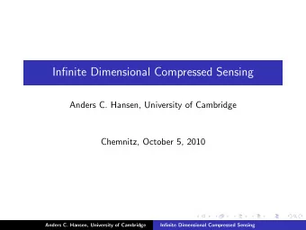
Compressed sensing in the real world - The need for a new theory Anders C. Hansen (Cambridge) Joint work with: B. Adcock (Purdue) C. Poon (Cambridge) B. Roman (Cambridge) Paris, January 13, 2014 1 / 49

Compressed Sensing in Inverse Problems Typical analog/infinite-dimensional inverse problem where compressed sensing is/can be used: (i) Magnetic Resonance Imaging (MRI) (ii) X-ray Computed Tomography (iii) Thermoacoustic and Photoacoustic Tomography (iv) Single Photon Emission Computerized Tomography (v) Electrical Impedance Tomography (vi) Electron Microscopy (vii) Reflection seismology (viii) Radio interferometry (ix) Fluorescence Microscopy 2 / 49

Compressed Sensing in Inverse Problems Most of these problems are modelled by the Fourier transform � R d f ( x ) e − 2 π i ω · x dx , F f ( ω ) = or the Radon transform R f : S × R → C (where S denotes the circle) � R f ( θ, p ) = f ( x ) dm ( x ) , � x ,θ � = p where dm denotes Lebesgue measure on the hyperplane { x : � x , θ � = p } . ◮ Fourier slice theorem ⇒ both problems can be viewed as the problem of reconstructing f from pointwise samples of its Fourier transform. f ∈ L 2 ( R d ) . g = F f , (1) 3 / 49

Compressed Sensing ◮ Given the linear system Ux 0 = y . ◮ Solve min � z � 1 subject to P Ω Uz = P Ω y , where P Ω is a projection and Ω ⊂ { 1 , . . . , N } is subsampled with | Ω | = m . If m ≥ C · N · µ ( U ) · s · log( ǫ − 1 ) · log ( N ) . then P ( z = x 0 ) ≥ 1 − ǫ , where i , j | U i , j | 2 µ ( U ) = max is referred to as the incoherence parameter. 4 / 49

Pillars of Compressed Sensing ◮ Sparsity ◮ Incoherence ◮ Uniform Random Subsampling In addition: The Restricted Isometry Property + uniform recovery. Problem: These concepts are absent in virtually all the problems listed above. Moreover, uniform random subsampling gives highly suboptimal results. Compressed sensing is currently used with great success in these fields, however the current theory does not cover this. 5 / 49

Uniform Random Subsampling U = U dft V − 1 dwt . 5% subsamp-map Reconstruction Enlarged 6 / 49

Sparsity ◮ The classical idea of sparsity in compressed sensing is that there are s important coefficients in the vector x 0 that we want to recover. ◮ The location of these coefficients is arbitrary. 7 / 49

Sparsity and the Flip Test Let x = and A = P Ω U df V − 1 y = U df x , dw , where P Ω is a projection and Ω ⊂ { 1 , . . . , N } is subsampled with | Ω | = m . Solve min � z � 1 subject to Az = P Ω y . 8 / 49

Sparsity - The Flip Test 2 1.5 Truncated (max = 151.58) 1 0.5 0 x10 5 1 2 3 4 5 6 7 8 9 10 Figure: Wavelet coefficients and subsampling reconstructions from 10% of Fourier coefficients with 2 ) − 1 and (1 + ω 2 distributions (1 + ω 2 1 + ω 2 1 + ω 2 2 ) − 3 / 2 . If sparsity is the right model we should be able to flip the coefficients. Let 2 Truncated (max = 151.58) 1.5 z f = 1 0.5 0 1 2 3 4 5 6 7 8 9 10 x10 5 9 / 49

Sparsity - The Flip Test ◮ Let y = U df V − 1 ˜ dw z f ◮ Solve min � z � 1 subject to Az = P Ω ˜ y to get ˆ z f . x = V − 1 ◮ Flip the coefficients of ˆ z f back to get ˆ z , and let ˆ dw ˆ z . ◮ If the ordering of the wavelet coefficients did not matter i.e. sparsity is the right model, then ˆ x should be close to x . 10 / 49

Sparsity- The Flip Test: Results Figure: The reconstructions from the reversed coefficients. Conclusion: The ordering of the coefficients did matter. Moreover, this phenomenon happens with all wavelets, curvelets, contourlets and shearlets and any reasonable subsampling scheme. Question: Is sparsity really the right model? 11 / 49

Sparsity - The Flip Test CS reconstr. CS reconstr, w/ flip Subsampling coeffs. pattern 512, 20% U Had V − 1 dwt Fluorescence Microscopy 1024, 12% U Had V − 1 dwt Compressive Imaging, Hadamard Spectroscopy 12 / 49

Sparsity - The Flip Test (contd.) CS reconstr. CS reconstr, w/ flip Subsampling coeffs. pattern 1024, 20% U dft V − 1 dwt Magnetic Resonance Imaging 512, 12% U dft V − 1 dwt Tomography, Electron Microscopy 13 / 49

Sparsity - The Flip Test (contd.) CS reconstr. CS reconstr, w/ flip Subsampling coeffs. pattern 1024, 10% U dft V − 1 dwt Radio interferometry 14 / 49

What about the RIP? ◮ Did any of the matrices used in the examples satisfy the RIP? 15 / 49

Images are not sparse, they are asymptotically sparse How to measure asymptotic sparsity: Suppose ∞ � f = β j ϕ j . j =1 Let � N = { M k − 1 + 1 , . . . , M k } , k ∈ N where 0 = M 0 < M 1 < M 2 < . . . and { M k − 1 + 1 , . . . , M k } is the set of indices corresponding to the k th scale. Let ǫ ∈ (0 , 1] and let K M k � � � � � � � � s k := s k ( ǫ ) = min K : β π ( i ) ϕ π ( i ) � ≥ ǫ β j ϕ j , � � � � � � � i =1 i = M k − 1 +1 in order words, s k is the effective sparsity at the k th scale. Here π : { 1 , . . . , M k − M k − 1 } → { M k − 1 + 1 , . . . , M k } is a bijection such that | β π ( i ) | ≥ | β π ( i +1) | . 16 / 49

Images are not sparse, they are asymptotically sparse 1 1 Level 1 Level 1 Level 2 Level 2 Sparsity, s k ( ǫ ) / ( M k − M k − 1 ) Sparsity, s k ( ǫ ) / ( M k − M k − 1 ) Level 3 Level 3 0.8 0.8 Level 4 Level 4 Level 5 Level 5 Level 6 Level 6 Level 7 Level 7 0.6 0.6 Level 8 Level 8 Worst sparsity Worst sparsity Best sparsity Best sparsity 0.4 0.4 0.2 0.2 0 0 0 0.2 0.4 0.6 0.8 1 0 0.2 0.4 0.6 0.8 1 Relative threshold, ǫ Relative threshold, ǫ Figure: Relative sparsity of Daubechies 8 wavelet coefficients. 17 / 49

Images are not sparse, they are asymptotically sparse 1 1 Level 1 Level 1 Level 2 Level 2 Sparsity, s k ( ǫ ) / ( M k − M k − 1 ) Sparsity, s k ( ǫ ) / ( M k − M k − 1 ) Level 3 Level 3 0.8 0.8 Level 4 Level 4 Level 5 Level 5 Level 6 Level 6 Level 7 Level 7 0.6 0.6 Worst sparsity Worst sparsity Curvelets Best sparsity Best sparsity 0.4 0.4 0.2 0.2 0 0 0 0.2 0.4 0.6 0.8 1 0 0.2 0.4 0.6 0.8 1 Relative threshold, ǫ Relative threshold, ǫ 1 1 Level 1 Level 1 Level 2 Level 2 Sparsity, s k ( ǫ ) / ( M k − M k − 1 ) Sparsity, s k ( ǫ ) / ( M k − M k − 1 ) Level 3 Level 3 0.8 0.8 Level 4 Level 4 Level 5 Level 5 Level 6 Level 6 Worst sparsity Worst sparsity 0.6 0.6 Best sparsity Best sparsity Contourlets 0.4 0.4 0.2 0.2 0 0 0 0.2 0.4 0.6 0.8 1 0 0.2 0.4 0.6 0.8 1 Relative threshold, ǫ Relative threshold, ǫ 1 1 Level 1 Level 1 Level 2 Level 2 Sparsity, s k ( ǫ ) / ( M k − M k − 1 ) Sparsity, s k ( ǫ ) / ( M k − M k − 1 ) Level 3 Level 3 0.8 0.8 Level 4 Level 4 Level 5 Level 5 Worst sparsity Worst sparsity Best sparsity Best sparsity 0.6 0.6 Shearlets 0.4 0.4 0.2 0.2 0 0 0 0.2 0.4 0.6 0.8 1 0 0.2 0.4 0.6 0.8 1 Relative threshold, ǫ Relative threshold, ǫ 18 / 49

Analog inverse problems are coherent Let U n = U df V − 1 dw ∈ C n × n where U df is the discrete Fourier transform and V dw is the discrete wavelet transform. Then µ ( U n ) = 1 for all n and all Daubechies wavelets! 19 / 49

Analog inverse problems are coherent, why? Note that U df V − 1 WOT-lim dw = U , n →∞ where   � ϕ 1 , ψ 1 � � ϕ 2 , ψ 1 � · · · � ϕ 1 , ψ 2 � � ϕ 2 , ψ 2 � · · · U =  .   . .  ... . . . . Thus, we will always have µ ( U df V − 1 dw ) ≥ c . 20 / 49

Analog inverse problems are asymptotically incoherent Fourier to DB4 Fourier to Legendre Polynomials Figure: Plots of the absolute values of the entries of the matrix U 21 / 49

Hadamard and wavelets are coherent Let U n = HV − 1 dw ∈ C n × n where H is a Hadamard matrix and V dw is the discrete wavelet transform. Then µ ( U n ) = 1 for all n and all Daubechies wavelets! 22 / 49

Hadamard and wavelets are asymptotically incoherent Hadamard to Haar Hadamard to DB8 23 / 49

We need a new theory ◮ Such theory must incorporates asymptotic sparsity and asymptotic incoherence. ◮ It must explain the two intriguing phenomena observed in practice: ◮ The optimal sampling strategy is signal structure dependent ◮ The success of compressed sensing is resolution dependent ◮ The theory cannot be RIP based (at least not with the classical definition of the RIP) 24 / 49

Sparsity in levels Definition For r ∈ N let M = ( M 1 , . . . , M r ) ∈ N r with 1 ≤ M 1 < . . . < M r and s = ( s 1 , . . . , s r ) ∈ N r , with s k ≤ M k − M k − 1 , k = 1 , . . . , r , where M 0 = 0. We say that β ∈ l 2 ( N ) is ( s , M )-sparse if, for each k = 1 , . . . , r , ∆ k := supp ( β ) ∩ { M k − 1 + 1 , . . . , M k } , satisfies | ∆ k | ≤ s k . We denote the set of ( s , M )-sparse vectors by Σ s , M . 25 / 49

Sparsity in levels Definition j ∈ N β j ϕ j ∈ H , where β = ( β j ) j ∈ N ∈ l 1 ( N ). Let Let f = � σ s , M ( f ) := min � β − η � l 1 . (2) η ∈ Σ s , M 26 / 49