Complex models - large p, small n Shrinkage estimation Applying - PDF document

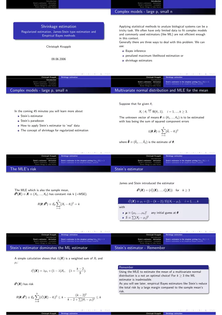
Introduction Introduction Stein’s estimator - derivation Stein’s estimator - derivation Stein’s estimator - examples Stein’s estimator - examples Some things to take home Some things to take home Complex models - large p, small n Shrinkage estimation Applying statistical methods to analyze biological systems can be a tricky task. We often have only limited data to fit complex models Regularized estimation, James-Stein type estimation and and commonly used estimators (like ML) are not efficient enough Empirical Bayes methods in this context. Generally there are three ways to deal with this problem. We can use: Christoph Knappik Bayes inference penalized maximum likelihood estimation or 09.06.2006 shrinkage estimators Christoph Knappik Shrinkage estimation Christoph Knappik Shrinkage estimation Introduction Introduction Stein’s estimator - derivation Stein’s estimator - derivation Stein’s estimator in the simplest setting: Var θ i ( X i ) = 1 Stein’s estimator - examples Stein’s estimator - examples Stein’s estimator in an empirical Bayes context Some things to take home Some things to take home Complex models - large p, small n Multivariate normal distribution and MLE for the mean Suppose that for given θ i ind In the coming 45 minutes you will learn more about X i | θ i ∼ N ( θ i , 1) , i = 1 , ..., k ≥ 3 . Stein’s estimator The unknown vector of means θ θ θ ≡ ( θ 1 , ..., θ k ) is to be estimated Stein’s paradoxon with loss being the sum of squared component errors How to apply Stein’s estimator to ’real’ data k � The concept of shrinkage for regularized estimation θ, ˆ (ˆ θ i − θ i ) 2 L ( θ θ θ θ θ ) ≡ i =1 where ˆ θ ≡ (ˆ ˆ ˆ θ 1 , ..., ˆ θ θ θ θ k ) is the estimate of θ θ . Christoph Knappik Shrinkage estimation Christoph Knappik Shrinkage estimation Introduction Introduction Stein’s estimator - derivation Stein’s estimator in the simplest setting: Var θ i ( X i ) = 1 Stein’s estimator - derivation Stein’s estimator in the simplest setting: Var θ i ( X i ) = 1 Stein’s estimator - examples Stein’s estimator in an empirical Bayes context Stein’s estimator - examples Stein’s estimator in an empirical Bayes context Some things to take home Some things to take home The MLE’s risk Stein’s estimator James and Stein introduced the estimator δ 1 δ 1 δ 1 ( X X ) = ( δ 1 X ) , ..., δ 1 The MLE which is also the sample mean, X 1 ( X X k ( X X )) X for k ≥ 3 δ 0 δ 0 δ 0 ( X X X ) ≡ X X X ≡ ( X 1 , ..., X k ) has constant risk k (=MSE). δ 1 k i ( X X ) ≡ µ i + (1 − ( k − 2) / S )( X i − µ i ) , X i = 1 , ..., k � ( X i − θ i ) 2 = k θ,δ 0 δ 0 δ 0 ) ≡ E θ θ R ( θ with i =1 µ µ ≡ ( µ 1 , ..., µ k ) ′ θ µ any initial guess at θ θ S ≡ � ( X j − µ j ) 2 Christoph Knappik Shrinkage estimation Christoph Knappik Shrinkage estimation Introduction Introduction Stein’s estimator in the simplest setting: Var θ i ( X i ) = 1 Stein’s estimator in the simplest setting: Var θ i ( X i ) = 1 Stein’s estimator - derivation Stein’s estimator - derivation Stein’s estimator - examples Stein’s estimator in an empirical Bayes context Stein’s estimator - examples Stein’s estimator in an empirical Bayes context Some things to take home Some things to take home Stein’s estimator dominates the ML estimator Stein’s estimator - Remember A simple calculation shows that δ i ( X X X ) is a weighted sum of X i and µ i : Remember ( λ = k − 2 δ 1 i ( X X ) = λµ i + (1 − λ ) X i , X ) . Using the MLE to estimate the mean of a multivariate normal S distribution is a not an optimal choice! For k ≥ 3 the ML estimator is inadmissible. δ 1 ( X δ 1 δ 1 As you will see later, empirical Bayes estimators like Stein’s reduce X X ) has risk the total risk by a large margin compared to the sample mean’s risk. k ( k − 2) 2 � X ) − θ i ) 2 ≤ k − θ,δ 1 δ 1 ) ≡ E θ δ 1 ( δ 1 R ( θ θ i ( X X k − 2 + � ( θ i − µ i ) 2 ≤ k i =0 Christoph Knappik Shrinkage estimation Christoph Knappik Shrinkage estimation

Introduction Introduction Stein’s estimator - derivation Stein’s estimator in the simplest setting: Var θ i ( X i ) = 1 Stein’s estimator - derivation Stein’s estimator in the simplest setting: Var θ i ( X i ) = 1 Stein’s estimator - examples Stein’s estimator in an empirical Bayes context Stein’s estimator - examples Stein’s estimator in an empirical Bayes context Some things to take home Some things to take home Stein’s estimator in an empirical Bayes context The empirical Bayes context - a priori and a posteriori distribution of θ i δ 1 i ( X X ) ≡ µ i + (1 − ( k − 2) / S )( X i − µ i ) , X i = 1 , ..., k arises quite naturally in an empirical Bayes context. If the { θ i } themselves are a sample from a prior distribution, ind ∼ N ( µ i , τ 2 ) , θ i i = 1 , ..., k then the Bayes estimate of θ i is the a posteriori mean of θ i given the data i ( X i ) = E θ i | X i = µ i + (1 − (1 + τ 2 ) − 1 δ ∗ )( X i − µ i ) � �� � λ Christoph Knappik Shrinkage estimation Christoph Knappik Shrinkage estimation Introduction Introduction Stein’s estimator - derivation Stein’s estimator in the simplest setting: Var θ i ( X i ) = 1 Stein’s estimator - derivation Stein’s estimator in the simplest setting: Var θ i ( X i ) = 1 Stein’s estimator - examples Stein’s estimator in an empirical Bayes context Stein’s estimator - examples Stein’s estimator in an empirical Bayes context Some things to take home Some things to take home The empirical Bayes context - estimation of τ 2 The empirical Bayes context - derivation of Stein’s estimator In the empirical Bayes situation τ 2 is unknown but it can be Substitution of ( k − 2) / S for the unknown 1 / (1 + τ 2 ) in estimated because marginally the { X i } are independently normal with means { µ i } and i ( X i ) = E θ i | X i = µ i + (1 − (1 + τ 2 ) − 1 )( X i − µ i ) δ ∗ � ( X j − µ j ) 2 ∼ (1 + τ 2 ) χ 2 S = results in k µ i + (1 − ( k − 2) / S )( X i − µ i ) ≡ δ 1 Since k ≥ 3, the unbiased estimate i ( X X ) X E ( k − 2) / S = 1 / (1 + τ 2 ) δ 1 i ( X X X ) has risk X ) − θ i ) 2 = 1 − ( k − 2) / k (1 + τ 2 ) is available. E τ E θ ( δ 1 i ( X X Christoph Knappik Shrinkage estimation Christoph Knappik Shrinkage estimation Introduction Introduction Stein’s estimator - derivation Stein’s estimator in the simplest setting: Var θ i ( X i ) = 1 Stein’s estimator - derivation Stein’s estimator in the simplest setting: Var θ i ( X i ) = 1 Stein’s estimator - examples Stein’s estimator in an empirical Bayes context Stein’s estimator - examples Stein’s estimator in an empirical Bayes context Some things to take home Some things to take home The empirical Bayes context - Stein’s estimator’s risk The empirical Bayes context - positive part Stein X ) − θ i ) 2 = 1 − ( k − 2) / k (1 + τ 2 ) E τ E θ ( δ 1 A simple way to improve δ 1 i is to use min { 1 , ( k − 2) / S } as an i ( X X estimate of 1 / (1 + τ 2 ) instead of E ( k − 2) / S . is to be compared to the corresponding risks of This results in δ 1+ 1 for the MLE and X ) = µ i + (1 − ( k − 2) / S ) + ( X i − µ i ) ( X X i 1 − 1 / (1 + τ 2 ) for the Bayes estimator with a + ≡ max (0 , a ). Thus if k is moderate or large δ 1 i is nearly as good as the Bayes δ 1+ δ 1 θ,δ 1+ δ 1+ ) < R ( θ θ,δ 1 δ 1 ) It can be proofed that R ( θ θ θ ∀ θ θ θ . estimator, but it avoids the possible gross errors of the Bayes estimator if τ 2 is misspecified. Christoph Knappik Shrinkage estimation Christoph Knappik Shrinkage estimation Introduction Introduction Stein’s estimator in the simplest setting: Var θ i ( X i ) = 1 Stein’s estimator - derivation Stein’s estimator - derivation Baseball data - Stein’s estimator as shrinkage estimator Stein’s estimator - examples Stein’s estimator in an empirical Bayes context Stein’s estimator - examples Some things to take home Some things to take home The empirical Bayes context - Remember Using Stein’s estimator to predict batting averages Remember Stein’s estimator dominates the MLE for k ≥ 3 Stein’s estimator can be interpreted as an empirical Bayes estimator Christoph Knappik Shrinkage estimation Christoph Knappik Shrinkage estimation