Comparing Seasonal Forecasts of Industrial Production Pedro - - PowerPoint PPT Presentation

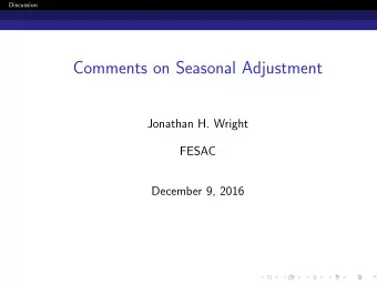
Conference on Seasonality, Seasonal Adjustment and their implications for Short-Term Analysis and Forecasting

10-12 May 2006

Comparing Seasonal Forecasts of Industrial Production

Pedro M.D.C.B. Gouveia Denise R Osborn Paulo M.M. Rodrigues

Comparing Seasonal Forecasts of Industrial Production Pedro M.D.C.B. Gouveia

University of Algarve

Denise R Osborn

University of Manchester

Paulo M.M. Rodrigues

University of Algarve

Invited presentation by Denise Osborn at Eurostat conference “Seasonality, Seasonal Adjustment and their Implications for Short-Term Analysis and Forecasting”, Luxembourg 10-12 May 2006.

• 1. Background

Short run properties of many economic time series dominated by

seasonality;

Particularly true of industrial production in some European countries; Various methods are available for modelling seasonality; Forecasting now embodied in X-12-ARIMA seasonal adjustment; But little investigation of forecast accuracy for seasonal series.

2

Recent interest in forecasting using combination methods. Two advantages:

• 1. Improved accuracy compared to individual models;
• 2. Less risky than selecting a specific model.

Indeed, simple mean of individual forecasts often performs well. This paper studies forecast performance for monthly industrial production:

Individual models and combinations Combinations may exploit different approaches to seasonal modelling

3

We consider:

17 individual forecasting models 18 forecast combination methods

Issues of interest:

• 1. Do some classes of methods perform better than others?
• 2. Do combinations improve forecast accuracy?
• 3. Are some combination methods better than others?

4

• 2. Data

Seasonally unadjusted industrial production indices for 17 countries:

Austria, Canada, Denmark, Finland, France, Germany, Greece, Hungary, Italy, Japan, Luxembourg, Netherlands, Portugal, Spain, Sweden, UK, USA Plus Euro Area

Data:

January 1980 to December 2005 Estimation & modelling: January 1980 to December 2002 Forecast period: January 2003 to December 2005

Outliers (estimation period) removed using Tramo/Seats

5

Descriptive Statistics (Selected Series) Annual Growth (%) Monthly Growth (%) Country Mean

• St. Dev.

Mean

• St. Dev.

France 1.14 3.15 0.08 15.13 Germany 1.37 3.37 0.10 6.71 Italy 0.90 4.36 0.06 31.85 UK 1.00 3.52 0.06 7.14 USA 2.52 3.67 0.21 2.01 Euro Area 1.55 3.09 0.12 11.12 Annual/monthly standard deviations reflect different strengths of seasonality.

6

• 3. Models

Observation for "season" (month) s of year n: ySn+s, s = 1,...,S; n = 0, 1, ... with S = 12 for monthly data. Models for seasonal ySn+s can be classified in various ways. We consider: Linear models of ARMA class; Nonlinear threshold models; Periodic (seasonally varying coefficient) models.

7

Linear Models Linear models are based on: ySn+s = µSn+s + xSn+s φ(L) xSn+s = uSn+s where: µSn+s = E[ySn+s] is trend & seasonals, φ(L) embodies any nonstationarity, uSn+s is stationary, β(L) uSn+s = θ(L) εSn+s Different linear models make different assumptions about φ(L).

8

Framework: ySn+s = µSn+s + xSn+s φ(L) xSn+s = uSn+s Seasonally integrated model Assumes seasonal nonstationarity: φ(L) = 1 – LS = ∆S = (1 – L)(1 + L + … + LS-1) S unit roots; seasons not cointegrated. Roots of 1 + L + … + LS-1 are seasonal unit roots.

9

Deterministic seasonal model Stationary seasonality (no seasonal unit roots): φ(L) = 1, or = 1 – L SARIMA model Seasonal and first differences: φ(L) = ∆S∆1 = (1 – L)2 (1 + L + … + LS-1) Two zero frequency unit roots plus seasonal unit roots.

10

Evidence of nonstationarity May be able to discriminate between linear models through (seasonal) unit root tests. HEGY-type test based on ∆S = (1 – L) (1 + L + … + LS-1) t0 tests conventional unit root (first differencing) F1…6 tests seasonal unit roots (1 + L + … + LS-1) F0…6 tests first and seasonal unit roots (annual differencing)

11

Seasonal Unit Root Tests (* Significant at 5%) t0 F1…6 F0…6 Implication France * * ∆1 Germany ∆12 Italy ∆12 UK * * ∆1 USA * * ∆1 Euro Area ∆12 Overall:

• Reject seasonal unit roots for about half of series;
• Support seasonal integration for a group of European countries

(Finland, Germany, Greece, Italy, Portugal, Spain, and Euro Area);

• Strongest evidence against seasonal integration for UK & USA;
• Conventional unit root supported for all series.

12

Nonlinear SETAR Models SETAR is AR model with regime-dependent coefficients ySn+s = ∑αs,jDs,Sn+s + φ1,j ySn+s-1 + … + φp,j ySn+s-p + εSn+s,j, j = 1, 2 Ds,Sn+s are seasonal dummy variables and regime j is determined by j = 1 if ∆SySn+s-d ≤ γ j = 2 if ∆SySn+s-d > γ with γ and d unknown. Test for nonlinearity, with max p of 12 and d ≤ p, via bootstrap. Null hypothesis is linearity, or same coefficients for j = 1, 2.

13

Linearity Tests γ d p-value France .019 8 .167 Germany .037 5 .007* Italy .078 12 .112 UK .045 1 .129 USA

• .051

2 .067 Euro Area .014 10 .001* Overall: Reject linearity (5%) for about half of series.

14

Periodic Models Periodic models allow coefficients to change with the seasons. PAR(p): ySn+s = αsDs,Sn+s + φ1,s ySn+s-1 + … + φp,s ySn+s-p + εSn+s, s = 1, …, 12 with not all φi,1 = … = φi,S = φi, i = 1, …, p Can test for periodic variation either directly on the coefficients, or using residuals from a non-periodic model. S = 12 seasons may be excessive; also group months to construct S = 3 “seasons” (negative, low positive, high positive average monthly growth).

15

Periodicity Tests (* Significant at 5%) Coefficient Tests Residual Tests PAR(3) PAR(12) PAR(3) PAR(12) France * * * * Germany * * * Italy * * * UK * * * USA * * * * Euro Area * * * Overall: evidence of periodic coefficients for all series.

16

Summary:

Mixed evidence about appropriate differences (first or annual) Mixed evidence about presence of nonlinearity Strong evidence for seasonally-varying autoregressive coefficients

Nevertheless, apply all models to all series.

17

• 4. Forecast Accuracy

Use m post-sample observations to evaluate h-step ahead forecasts from models fitted to the first T observations. Accuracy measured by Root Mean Squared Predic- tion Error (RMSPE)

RMSPE(h) = v u u t 1 m − h + 1

T+m

X

j=h

¡ b yT+j|T+j−h − yT+j ¢2

Nonlinear model forecasts computed using bootstrap. Forecast Combination Methods Can be simple measures (mean, median),

• r more sophisticated methods based on perfor-

mance.

Historical RMSPE Combine k separate h-step forecasts, b

yi

Sn+s+h|Sn+s

(i = 1, ..., k) as

b yc

Sn+s+h|Sn+s = k

X

i=1

wh

i b

yi

Sn+s+h|Sn+s

with weight wh

i

wh

i = [1/RMSPE(h)i]λ/ k

X

j=1

[1/RMSPE(h)i]λ

for λ ∈ {0, 1, 1.25, 1.5, 2}.

RMSPE(h)i computed using estimation period b yi

T−35|T−35−h to b

yi

T|T−h.

Also use discounted RMSPE weights

wh

i =

¡ mh

i

¢−1 /

k

X

j=1

¡ mh

j

¢−1

where

mh

i =

v u u t

T−h

X

j=1

δj−1 ³ b yi

T−j+1|T−j+1−h − yT−j+1

´2

for discount factor δ ∈ {1, 0.95, 0.90}.

Regression Methods Weights determined from

ySn+s+h = β0 +

k

X

j=1

βjb yj

Sn+s+h|Sn+s + εSn+s+h

estimated using observations yT−35 to yT. In practice, only best 5 forecasts used.

• 5. Forecast Performance

Methods Employed Forecast Models Code Individual Models Filter Deterministic terms M1

ARMA(1, 1) ∆12

Intercept M2

ARMA(2, 2) ∆12

Intercept M3

ARMA(3, 3) ∆12

Intercept M4

AR(p) ∆12

Intercept M5

SETAR (p1,p2) ∆12

Intercept M6

AR (p) levels Seas. intercepts + trend

M7

PAR(12, 3) levels Seas. intercepts + trend

M8

PAR(3, 3) levels Seas. intercepts & trends

M9

SETAR(p1, p2) levels Seasonal intercepts

M10 AR (p)

∆1

Seasonal intercepts M11 PAR(3, 3)

∆1

• Seas. intercepts + trend

M12 PAR(12, 3)

∆1

• Seas. intercepts & trends

M13 SETAR(p1, p2)

∆1

Seasonal intercepts M14 ARMA(1, 1)

∆1∆12 None

M15 ARMA(2, 2)

∆1∆12 None

M16 ARMA(3, 3)

∆1∆12 None

M17 AR(p)

∆1∆12 None

Combination Methods Code Combination method parameters C1 mean of M1 to M17 C2 median of M1 to M17 C3 RMSPE weight

λ = 0

C4 RMSPE weight

λ = 1

C5 RMSPE weight

λ = 1.25

C6 RMSPE weight

λ = 1.5

C7 RMSPE weight

λ = 2

C8 mean of best 5 models C9 mean of best 10 models C10 mean of best 15 models C11 median of best 5 models C12 median of best 10 models C13 median of best 15 models C14 discounted RMSPE weight

δ = 1

C15 discounted RMSPE weight

δ = 0.95

C16 discounted RMSPE weight

δ = 0.9

C17 regression weight C18 mean of combinations

Results Forecast Accuracy for Euro Area

h = 1 h = 3 h = 8 Rank Method RMSPE Method RMSPE Method RMSPE 1 PAR(12, 3) levels 0.0187 Median (best 5) 0.0304 ARMA(2, 2) ∆12 0.0545 2 PAR(3, 3) ∆1 0.0195 AR(p) ∆12 0.0304 Mean (all models) 0.0552 3 AR(p) ∆1 0.0196 PAR(12, 3) ∆1 0.0305 ARMA(3, 3) ∆12 0.0561 4 Mean (all models) 0.0198 Median (all models) 0.0307 Median (best 10) 0.0561 5 Discounted RMSPE δ = 0.9 0.0199 PAR(3,3) levels 0.0311 Median (all models) 0.0564

23

Forecast Accuracy for USA h = 1 h = 3 h = 8 Rank Method RMSPE Method RMSPE Method RMSPE 1 AR(p) ∆1 0.0086 Median (best 5) 0.0143 AR(p) ∆1 0.0302 2 Mean (best 5) 0.0087 Mean (all models) 0.0144 PAR(3, 3) ∆1 0.0310 3 Median (best 5) 0.0087 AR(p) ∆1 0.0145 Median (best 5) 0.0329 4 AR(p) levels 0.0087 PAR(12, 3) levels 0.0146 RMSPE wt. (no discount) 0.0335 5 Median (best 10) 0.0087 Mean (best 5) 0.0147 Median (best 10) 0.0336

24

Average Rank and Relative RMSPE (Selected Models) h = 1 h = 3 h = 8 Method Rank Relative Rank RMSPE Relative RMSPE Rank Relative RMSPE ARMA(1, 1) ∆12 22 1.000 20 1.000 18 1.000 AR(p) ∆1 18 0.945 18 0.975 21 1.077 AR(p) ∆12 22 0.981 19 0.998 21 1.078 AR(p) ∆1∆12 21 0.967 20 0.995 22 1.096 SETAR(p1, p2) ∆12 27 1.035 30 1.199 26 1.303 PAR(12, 3) ∆1 24 1.037 19 1.046 24 1.091

25

Average Rank and Relative RMSPE (Selected Combination Methods) h = 1 h = 3 h = 8 Method Rank Relative Rank RMSPE Relative RMSPE Rank Relative RMSPE Mean (all models) 11 0.910 17 1.023 11 0.980 Median (all models) 17 0.923 15 0.923 14 0.949 Mean (best 5) 9 0.908 17 1.093 17 1.013 Median (best 5) 11 0.912 13 0.926 16 1.006 Mean (best 10) 15 0.915 17 0.997 17 0.988 Median (best 10) 16 0.926 14 0.927 16 0.969

26

Average Rank and Relative RMSPE (Selected Combination Methods) h = 1 h = 3 h = 8 Method Rank Relative Rank RMSPE Relative RMSPE Rank Relative RMSPE Median (all models) 17 0.923 15 0.923 14 0.949 RMSPE weight (whole sample) 7 0.899 10 0.968 10 0.949 RMSPE weight λ = 1 10 0.903 9 0.945 9 0.947 RMSPE weight λ = 2 11 0.903 13 0.963 14 0.965 Discount RMSPE δ = 0.9 10 0.904 10 0.944 11 0.952 Regression based combination 11 0.904 11 0.945 13 0.956

27

• 6. Conclusions

Many different models proposed for seasonal data:

Seasonal (non)stationarity, nonlinearity, periodic coefficient variation;

For individual models, simple AR or ARMA models outperform

more complex ones (SETAR, PAR) for industrial production series.

Almost all combinations improve accuracy (in general) compared to

“best” individual model;

Simple mean/median combinations perform well for one-step ahead,

but less well for h > 1.

Best methods for h > 1 based on previous RMSPE, or overall

median forecast.

28