Verifjcatjon of Sub-seasonal to Seasonal Predictjons Caio Coelho - PowerPoint PPT Presentation

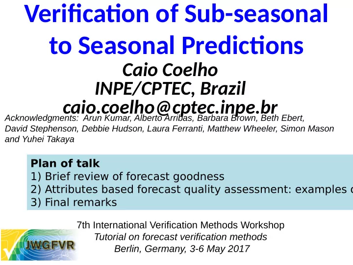
Verifjcatjon of Sub-seasonal to Seasonal Predictjons Caio Coelho INPE/CPTEC, Brazil caio.coelho@cptec.inpe.br Acknowledgments: Arun Kumar, Alberto Arribas, Barbara Brown, Beth Ebert, David Stephenson, Debbie Hudson, Laura Ferranti, Matthew Wheeler, Simon Mason and Yuhei Takaya Plan of talk 1) Brief review of forecast goodness 2) Attributes based forecast quality assessment: examples o 3) Final remarks 7th International Verification Methods Workshop Tutorial on forecast verification methods Berlin, Germany, 3-6 May 2017

What is a good forecast? Attributes of quality:  Association Good forecasts have:  Accuracy • QUALITY  Discrimination • VALUE/UTILITY  Reliability • CONSISTENCY  Resolution …  No single score can be used to summarize a set of forecasts A. H. Murphy 1993 “What is a good forecast ? An essay on the nature of goodness in weather forecasting” Weather and Forecasting, 8, 281-293.

Some defjnitjons • Quality: Measure of correspondence between forecasts and observatjons using mathematjcal relatjonship (deterministjc and probabilistjc scores) • Value: Measure of benefjt achieved (or loss incurred) through the use of forecasts • Consistency: Correspondence between a forecast and the forecasters belief. If consistent, the forecast must communicate what the forecaster thinks will happen, and correctly indicate the associated level of uncertainty

S2S forecast quality assessment 1. Atuributes of deterministjc forecasts (ensemble mean)

Associatjon • Overall strength of the relatjonship between the forecasts and observatjons • Linear associatjon is ofuen measured using the product moment correlatjon coeffjcient n   ( x - x )( y y ) i i  i  1 r n n   2 2 ( x - x ) ( y - y ) i i i  1 i  1 x: forecast y: observation n: number of (x,y) pairs

Relationship between past forecast and past obs. anomalies Observed anomalies (mm) y r = 0.54 Forecasts with positive association x Forecast anomalies (mm)

Relationship between past forecast and past obs. anomalies Observed anomalies (mm) y Slope=r*SD(y)/SD(x) Slope = 1 Slope < 1 r = 0.54 Var(y)<Var(x) Forecasts with positive association x Forecast anomalies (mm)

Accuracy • Average distance between forecasts and observatjons • Simplest measure is the Mean Error (Bias) x i - y i ME x: forecast y: observation n: number of (x,y) pairs

Seasonal forecast example: 1-month lead precip. fcsts for DJF

Monthly forecast example: 0-day lead precip. fcsts for next 30 days ACC (against GPCP v2 monthly) Bias (against GPCP v2 monthly) Day 1-30 mean Day 1-30 mean I.C. : Dec.-Feb. 1981-2010 I.C. : Dec.-Feb. 1981-2010 Yuhei Takaya, JMA

Monthly forecast example: 0, 5, 10 and 15-day lead fcsts for Feb Precipitation 2m Temperature Mingyue Chen NCEP/NOAA

Two weeks forecast example: ½ month lead precip. fcsts Correlation between forecast and observed precipitation anomalies Fortnight 2: Sep, Oct, Nov forecast start months. Hindcasts: 1980-2006 Debbie Hudson BOM, Australia

S2S forecast quality assessment 2. Atuributes of probabilistjc forecasts (derived from ensemble members)

Discriminatjon • Conditjoning of forecasts on observed outcomes • Addresses the questjon: Does the forecast difger given difgerent observed outcomes? Or, can the forecasts distjnguish an event from a non-event? • If the forecast is the same regardless of the outcome, the forecasts cannot discriminate an event from a non-event • Forecasts with no discriminatjon ability are useless because the forecasts are the same regardless of what happens

• The ROC curve is constructed by calculating the hit and f for various probability thresholds • Area under ROC curve (A) is a measure of discrimination successfully discriminating a warm (SST>0) from a cold (

Steep curve at bottom indicates forecasts with Shallow curve at high probabilities top indicates are good. forecasts with Good ability to low probabilities indicate that a are good. warm event Good ability to will occur. indicate that a warm event • The ROC curve is constructed by calculating the hit and f will not occur. for various probability thresholds • Area under ROC curve (A) is a measure of discrimination successfully discriminating a warm (SST>0) from a cold (

Seasonal forecast example: 1-month lead precip. fcsts for DJF ROC Skill Score = 2 A - 1

Monthly forecast example: 1-day lead 2mT fcsts for day 2-29 mean Relatjve Operatjng Characteristjcs T2m (upper tercile) Day 2-29 mean I.C. : Dec.-Feb. 1981- Yuhei Takaya, JMA 2010 N.H., TROP, S.H.

One to two weeks forecast example: Northern extratropics ROC score: 2-metre temperature in the upper tercile Monthly Forecast Monthly Forecast Persistence of day 5-18 Persistence of day 5-11 Day 19-32 (2 weeks) Day 12-18 (1 week ) Frederic Vitard and Laura Ferranti, ECMWF

Two weeks forecast example: ½ month lead precip. fcsts ROC area: Precipitation anomalies in the upper tercile Fortnight 2: Sep, Oct, Nov forecast start months. Hindcasts: 1980-2006 Debbie Hudson BOM, Australia

Reliability and resolutjon • Reliability: correspondence between forecast probabilities and observed relative frequency (e.g. an event must occur on 30% of the occasions that the 30% forecast probability was issued) • Resolution: Conditioning of observed outcome on the forecasts • Addresses the question: Does the frequency of occurrence of an event difgers as the forecast probability changes? • If the event occurs with the same relative frequency regardless of the forecast, the forecasts are said to have no resolution • Forecasts with no resolution are useless because the outcome is the same regardless of what is forecast

Reliability diagram Event: SST>0 (o i ) o N i 22 (p i )

Reliability diagram Blue dot: Climatological forecast (o i Perfectly reliable: Rel=0 ) Has no resolution: Res=0 . Event: SST>0 o N i 23 (p i )

Seasonal forecast example: 1-month lead MSLP fcsts for DJF GLOSEA5 Hindcast Probabilistic skill MSLP in N. Atlantic in upper and lower tercile Reliability ROC area MacLachlan et al., QJRMS, 2015

Monthly forecast example: 2-day lead 2mT fcsts for day 2-29 mean Reliability Diagrams T2m (upper tercile) Day 2-29 mean I.C. : Dec.-Feb. 1981- Yuhei Takaya, JMA 2010 N.H., TROP, S.H.

Two weeks forecast example: ½ month lead precip. fcsts Precipitation anomalies in the upper tercile Fortnight 2: Sep, Oct, Nov forecast start months. Hindcasts: 1980-2006 Debbie Hudson BOM, Australia

Seamless verifjcatjon Seamless forecasts - consistent across space/tjme scales single modelling system or blended probabilistjc / ensemble decadal climate seasonal sub- global change prediction seasonal prediction Spatial scale NWP prediction very regional short range Ebert, E., L. Wilson, A. Weigel, M. Mittermaier, P. Nurmi, local nowcasts P. Gill, M. Gober, S. Joslyn, B. Brown, T. Fowler, and A. Watkins, 2013: Progress and challenges in forecast verification . Meteorol. Appl. , 20, 130–139. point minutes hours days weeks months years decades forecast aggregation time

Final remarks • Clear need for attributes-based verification for a complete forecast quality view • Need for use more than a single score for more detailed forecast quality assessment • S2S verification is naturally leaning towards the seamless consistency concept addressing the question of which scales and phenomena are predictable • As S2S covers various forecast ranges (days, weeks and months) it naturally allows seamless verification developments

Thank you all for your attention!