Combining Partial Order Reduction with Bounded Model Checking CPA - PowerPoint PPT Presentation
Combining Partial Order Reduction with Bounded Model Checking CPA 2009 Jos e Vander Meulen and Charles Pecheur UC Louvain p. 1 A Concurrent System Set of asynchronous and interacting processes Producer 1 Consumer 1 Producer 2
Combining Partial Order Reduction with Bounded Model Checking CPA 2009 Jos´ e Vander Meulen and Charles Pecheur UC Louvain – p. 1
A Concurrent System • Set of asynchronous and interacting processes Producer 1 Consumer 1 Producer 2 Consumer 2 . . . . . . Producer q - 1 Consumer q - 1 bounded-buffer Producer q Consumer q • Can we verify this system with Symbolic Model Checking? • Up to what q ? – p. 2
Model Checking • Exhaustive exploration of the state space of a system – p. 3
Symbolic Model Checking • Principle: • Compute sets of states (BDDs), or • Resolve a SAT problem (BMC) • Brilliant results in the hardware domain [Biere + 03, Mc Millan 93] • Conventional wisdom: Symbolic Model Checking methods are not well suited for asynchronous systems. • How can we use symbolic Model Checking with asynchronous system? – p. 4
Outline • Background • Bounded Model Checking • Partial Order Reduction • Combining Partial Order Reduction with Bounded Model Checking • Experimental results • Conclusion • Perspectives – p. 5
Bounded Model Checking [ Biere + 99 ] • Search for a counterexample in executions whose length = k • e.g. paths of length 3 x y y z x y y z x y M x y y z x y z y z z x y y z z z x y z z z – p. 6
Bounded Model Checking [ Biere + 99 ] • Reduce model checking problem to a SAT problem • Unfold the transition relation k times to obtain a boolean formula [ [ M ] ] k I ( � x 0 ) ∧ T ( � x 1 ) ∧ T ( � x 2 ) ∧ · · · ∧ T ( � x k ) x 0 ,� x 1 ,� x k − 1 ,� • Translate the negation of a LTL property f to a Boolean formula [ [ ¬ f ] ] k • If [ [ M ] ] k ∧ [ [ ¬ f ] ] k is satisfiable, an error is found – p. 7
Partial Order Reduction • Partial order reduction methods are best suited for asynchronous systems • Can we use these methods with BMC and LTL? • Verification = only check some interleavings of a transition system • Based on independence x y between transitions and invisibility of a transition x ¬ y ¬ x y ¬ x ¬ y – p. 8
Partial Order Reduction • Partial order reduction methods are best suited for asynchronous systems • Can we use these methods with BMC and LTL? • Verification = only check some interleavings of a transition system • Based on independence x y between transitions and X invisibility of a transition X x ¬ y ¬ x y X ¬ x ¬ y – p. 9
Partial Order Reduction • Algorithm : modified depth-first search (DFS) • At each step s , a subset of the successors is selected: ample ( s ) • ample ( s ) has to respect a set of conditions • c1 : Along every path in the full state graph that starts at s : a transition that is dependent on a transition in ample ( s ) cannot be executed without a transition in ample ( s ) occurring first. x y x ¬ y ¬ x y ¬ x ¬ y x y – p. 10
Partial Order Reduction • c2 at least one state s per cycle is fully expanded • c3 If ample ( s ) � = enable ( s ) , all transitions in ample ( s ) are invisible. • c4 if ample ( s ) � = enable ( s ) , then ample ( s ) is a singleton • C1 – C3 preserve deadlocks, LTL X properties • C1 – C4 preserve CTL X properties – p. 11
Two-phase algorithm [Nalumasu + 97] • A modified DFS: performs alternatively 2 phases • Phase-1: explore for each process as many safe transitions ( C1, C4 ) as possible • Phase-2: fully expand the current state P 1 Phase 1 Safe transitions P 2 P 3 Phase 2 All transitions Phase 1 • Two-phase algorithm can check CTL X properties – p. 12
SBTP • Algorithm combining POR with BMC: • SBTP: Phase-1 performs a fixed number n of partial expansions for each process • A process might not be able to produce n safe transitions ( idle transitions) P 1 idle Phase 1 Safe transitions P 2 P 3 idle Phase 2 All transitions Phase 1 – p. 13
SBTP • From a transition system to a computation tree x y x y CT ( M ) M y z z y z z x y z z • M and CT ( M ) are equivalent – p. 14
SBTP • A modified computation tree ( ≈ CT ( M ) ) • Given p processes, a fixed number n of partial expansions, construct a reduced computation tree. • e.g number of processes p = 2 , and n = 3 T 0 else idle T 0 else idle T 0 else idle T 1 else idle SBTP ( M, n ) T 1 else idle T 1 else idle T T 0 else idle T 0 else idle T 0 else idle T 1 else idle T 1 else idle T 1 else idle T . . . – p. 15
SBTP • Given p processes, a fixed number n of partial expansions, and k = m ( p × n + 1) , apply m times the ] SBTP two phases to obtain [ [ M ] k,n • e.g number of processes p = 2 , and n = 3 � m � T idle T idle T idle T idle T idle T idle T 1 1 1 2 2 2 • Translate the negation of a LTL X property f to a boolean formula [ [ ¬ f ] ] k ] SBTP • If [ ] k is satisfiable, an error is found [ M ] ∧ [ [ ¬ f ] k,n – p. 16
Justification ] SBT P There exists k ≥ 0 such that [ [ M, ¬ f ] if and only if M �| = f k,n Our method finds a true assignment satisfying ¬ f ⇐ ⇒ Classical BMC on SBTP ( M, n ) finds a true assignment satisfying ¬ f ⇐ ⇒ SBTP ( M, n ) does not satisfy f ⇐ ⇒ M does not satisfy f – p. 17
Tool • Implemented in Scala: • Smoothly integrates features of object-oriented and functional languages. • Fully interoperable with Java. • SAT part uses the Yices SMT solver. • Main Features: • Modelling language based on processes and synchronization by rendezvous • BMC of LTL properties • SBTP of LTL X properties – p. 18
Case Study: Producer-Consumer • A variant of the Producer-Consumer problem: • with q producers, q consumers, and n = 8 • P 2 : in all cases the buffer will eventually contain more than one piece BMC property P 2 SBTP property P 2 states k sec k cycles sec q 1 1,059 26 73 153 9 122 2 51,859 44 29,898 297 9 211 3 3,807,747 — — 441 9 401 ≈ 10 8 4 — — 585 9 1,238 ≈ 10 10 5 — — 729 9 1,338 ≈ 10 12 6 — — 873 9 1,926 ≈ 10 14 7 — — 1,017 9 4,135 – p. 19
Case Study: Producer-Consumer • Influence of the parameter n when the number of producers (resp. consumers) = 2 property P 2 k # cycles TIME (sec) MEM (MB) n 0 44 44 29,898 131 1 95 19 855 159 2 135 15 235 167 3 169 13 305 194 4 187 11 217 192 5 231 11 375 308 6 275 11 381 240 7 319 11 583 318 8 297 9 211 224 9 333 9 240 295 – p. 20
Conclusion • Combining Partial Order Reduction with Bounded Model Checking • From 2 Producers/Consumers ( 51 , 859 states) to 7 Producers/Consumers ( ≈ 10 14 states) • How to choose the number n of partial expansions during Phase-1? • Need to apply SBTP to other case studies (more complex, more realistic) • Appropriate algorithm to check asynchronous systems with symbolic model-checking – p. 21
Perspectives • Extend SBTP to handle models featuring variables on infinite domains (SMT solvers) • Automatically determine the number n of partial expansions during Phase-1 • Consolidate our prototype: • Perform state-of-the-art BMC translations • Improve input language – p. 22
Recommend


More recommend
Explore More Topics
Stay informed with curated content and fresh updates.