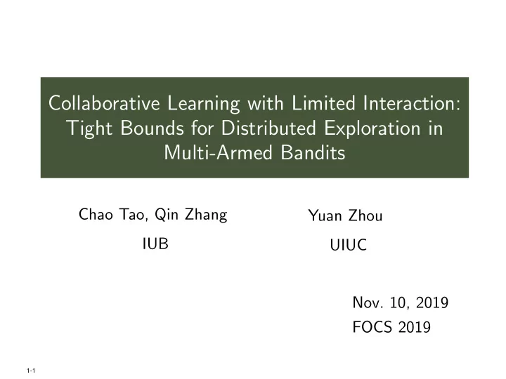
Collaborative Learning with Limited Interaction: Tight Bounds for - PowerPoint PPT Presentation

Collaborative Learning with Limited Interaction: Tight Bounds for Distributed Exploration in Multi-Armed Bandits Chao Tao, Qin Zhang Yuan Zhou IUB UIUC Nov. 10, 2019 FOCS 2019 1-1

Collaborative Learning One of the most important tasks in machine learning is to make learning scalable. 2-1

Collaborative Learning One of the most important tasks in machine learning is to make learning scalable. A natural way to speed up the learning process is to introduce multiple agents 2-2

Collaborative Learning with Limited Collaboration Interaction between agents can be expensive. 3-1

Collaborative Learning with Limited Collaboration Interaction between agents can be expensive. – Time: network bandwidth/latency, protocol handshaking – Energy: e.g., robots exploring in the deep sea and on Mars 3-2

Collaborative Learning with Limited Collaboration Interaction between agents can be expensive. – Time: network bandwidth/latency, protocol handshaking – Energy: e.g., robots exploring in the deep sea and on Mars Interested in tradeoffs between #rounds of interaction and the “speedup” of collaborative learning (to be defined shortly) 3-3

Best Arm Identification in Multi-Armed Bandits n alternative arms (randomly permuted), where the i -th arm is associated with an unknown reward distribution µ i with support on [0 , 1] Want to identify the arm with the largest mean Tries to identify the best arm by a sequence of arm pulls; each pull on the i -th arm gives an i.i.d. sample from µ i Goal (centralized setting): minimize total #arm-pulls 4-1

Best Arm Identification (cont.) Assume each arm pull takes one time step Fixed-time best arm : Given a time budget T , identify the best arm with the smallest error probability Fixed-confidence best arm : Given an error probability δ , identify the best arm with error probability at most δ using the smallest amount of time We consider both in this paper 5-1

Collaborative Best Arm Identification n alternative arms. K agents. P 1 P 2 P k Learning proceeds in rounds. 6-1

Collaborative Best Arm Identification n alternative arms. K agents. P 1 P 2 P k Learning proceeds in rounds. Each agent at any time, based on outcomes of all previous pulls, all comm. msgs received, and randomness of the algo, takes one of the followings comm. makes the next pull requests a comm. step and enters the wait mode terminates and outputs the answer. 6-2

Collaborative Best Arm Identification n alternative arms. K agents. P 1 P 2 P k Learning proceeds in rounds. Each agent at any time, based on outcomes of all previous pulls, all comm. msgs received, and randomness of the algo, takes one of the followings comm. makes the next pull requests a comm. step and enters the wait mode terminates and outputs the answer. A comm. step starts if all non-terminated agents are in the wait mode. After that agents start a new round of arm pulls 6-3

Collaborative Best Arm Identification (cont.) At the end, all agents need to output the same best arm 7-1

Collaborative Best Arm Identification (cont.) At the end, all agents need to output the same best arm Try to minimize – number of rounds R ; – running time T = � r ∈ [ R ] t r , where t r is the #time steps in the r -th round 7-2

Collaborative Best Arm Identification (cont.) At the end, all agents need to output the same best arm Try to minimize – number of rounds R ; – running time T = � r ∈ [ R ] t r , where t r is the #time steps in the r -th round Total cost of the algorithm: a weighted sum of R and T . Call for the best round-time tradeoffs 7-3

Speedup T A ( I , δ ): expected time needed for A to succeed on I with probability at least (1 − δ ). Speedup (of collaborative learning algorithms) T O ( I , δ ) β A ( T ) = inf inf inf T A ( I , δ ) centralized O instance I δ ∈ (0 , 1 / 3]: T O ( I ,δ ) ≤ T 8-1

Speedup T A ( I , δ ): expected time needed for A to succeed on I with probability at least (1 − δ ). Speedup (of collaborative learning algorithms) T O ( I , δ ) T (best cen) β A ( T ) = inf inf inf T ( A ) T A ( I , δ ) centralized O instance I δ ∈ (0 , 1 / 3]: T O ( I ,δ ) ≤ T 8-2

Speedup T A ( I , δ ): expected time needed for A to succeed on I with probability at least (1 − δ ). Speedup (of collaborative learning algorithms) T O ( I , δ ) T (best cen) β A ( T ) = inf inf inf T ( A ) T A ( I , δ ) centralized O instance I δ ∈ (0 , 1 / 3]: T O ( I ,δ ) ≤ T – Our upper bound slowly degrades (in log) as T grows 8-3

Speedup T A ( I , δ ): expected time needed for A to succeed on I with probability at least (1 − δ ). Speedup (of collaborative learning algorithms) T O ( I , δ ) β A ( T ) = inf inf inf T A ( I , δ ) centralized O instance I δ ∈ (0 , 1 / 3]: T O ( I ,δ ) ≤ T – Our upper bound slowly degrades (in log) as T grows β K , R ( T ) = sup A β A ( T ) where sup is taken over all R -round algorithms A for the collaborative learning model with K agents 8-4

Our Goal Find the best round-speedup tradeoffs Clearly there is a tradeoff between R and β K , R : • When R = 1 (i.e., no communication step), each agent needs to solve the problem by itself, and thus β K , 1 ≤ 1. • When R increases, β K , R may increase. • On the other hand we always have β K , R ≤ K . 9-1

Previous and Our Results [21]: Hillel et al. NIPS 2013; ∆ min = mean of best arm - mean of 2nd best arm 10-1

Previous and Our Results ˜ ln K Ω( K ) K / ln O (1) K Ω(ln K / ln ln K ) 1 ˜ ln Ω( K ) ∆ min � � K / ln O (1) K 1 1 Ω ln ∆ min / (ln ln K + ln ln ∆ min ) [21]: Hillel et al. NIPS 2013; ∆ min = mean of best arm - mean of 2nd best arm 10-2

Previous and Our Results ˜ ln K Ω( K ) K / ln O (1) K Ω(ln K / ln ln K ) 1 ˜ ln Ω( K ) ∆ min � � K / ln O (1) K 1 1 Ω ln ∆ min / (ln ln K + ln ln ∆ min ) [21]: Hillel et al. NIPS 2013; ∆ min = mean of best arm - mean of 2nd best arm Almost tight round-speedup tradeoffs for fixed-time. Today’s focus (LB) Almost tight round-speedup tradeoffs for fixed-confidence. A separation for two problems. 10-3

Previous and Our Results ˜ ln K Ω( K ) K / ln O (1) K Ω(ln K / ln ln K ) 1 ˜ ln Ω( K ) ∆ min � � K / ln O (1) K 1 1 Ω ln ∆ min / (ln ln K + ln ln ∆ min ) [21]: Hillel et al. NIPS 2013; ∆ min = mean of best arm - mean of 2nd best arm Almost tight round-speedup tradeoffs for fixed-time. Today’s focus (LB) Almost tight round-speedup tradeoffs for fixed-confidence. A separation for two problems. A generalization of the round-elimination technique. Today A new technique for instance-dependent round complexity. 10-4

Lower Bound: Fixed-Time 11-1

Round Elimination: A Technique for Round LB • ∃ an r -round algorithm with error prob. δ r and time budget T on an input distribution σ r , ⇒ ∃ an ( r − 1)-round algorithm with error prob. δ r − 1 ( > δ r ) and time budget T on an input distribution σ r − 1 . • There is no 0-round algorithm with error prob. δ 0 ≪ 1 on a nontrivial input distribution σ 0 . 12-1

Round Elimination: A Technique for Round LB • ∃ an r -round algorithm with error prob. δ r and time budget T on an input distribution σ r , ⇒ ∃ an ( r − 1)-round algorithm with error prob. δ r − 1 ( > δ r ) and time budget T on an input distribution σ r − 1 . • There is no 0-round algorithm with error prob. δ 0 ≪ 1 on a nontrivial input distribution σ 0 . ⇒ Any algo with time budget T and error prob. 0 . 01 needs at least r rounds of comm. 12-2

Previous Use of Round Elimination Agarwal et al. (COLT’17) used round elimination to prove an Ω(log ∗ n ) for best arm identification under � � time budget T = ˜ n min / K for non-adaptive algos O ∆ 2 – Translated into our collaborative learning setting – Non-adaptive algos: all arm pulls should be determined at the beginning of each round 13-1

Previous Use of Round Elimination Agarwal et al. (COLT’17) used round elimination to prove an Ω(log ∗ n ) for best arm identification under � � time budget T = ˜ n min / K for non-adaptive algos O ∆ 2 – Translated into our collaborative learning setting – Non-adaptive algos: all arm pulls should be determined at the beginning of each round “One-spike” distribution : a random single arm with � 1 mean 1 � 2 , and ( n − 1) arms with mean 2 − ∆ min . i ∗ (random index) 13-2

Previous Use of Round Elimination (Cont.) Basic argument (of COLT’17): If we do not make enough pulls in the first round, then conditioned on the pull outcomes, the index of the best arm is still quite uncertain 14-1

Previous Use of Round Elimination (Cont.) Basic argument (of COLT’17): If we do not make enough pulls in the first round, then conditioned on the pull outcomes, the index of the best arm is still quite uncertain More precisely, the posterior distribution of the index of the best arm can be written as a convex combination of a set of distributions, each of which has a large support size ( ≥ log n ) and is close to the uniform distribution 14-2