Coarse-graining dynamical networks and analysis of data collected - PowerPoint PPT Presentation
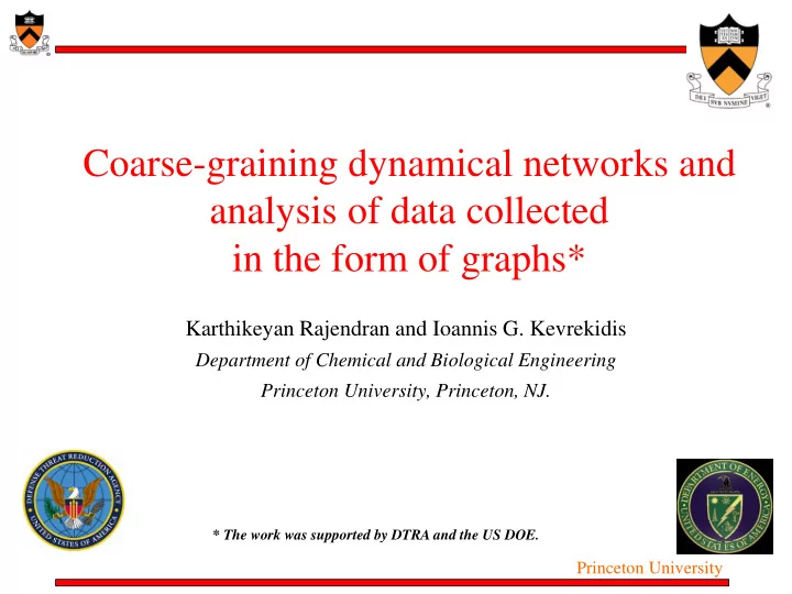
Coarse-graining dynamical networks and analysis of data collected in the form of graphs* Karthikeyan Rajendran and Ioannis G. Kevrekidis Department of Chemical and Biological Engineering Princeton University, Princeton, NJ. * The work was
Coarse-graining dynamical networks and analysis of data collected in the form of graphs* Karthikeyan Rajendran and Ioannis G. Kevrekidis Department of Chemical and Biological Engineering Princeton University, Princeton, NJ. * The work was supported by DTRA and the US DOE. Princeton University
Introduction Complex networks • Examples – Engineered (Internet) – Social (Facebook) – Biological (Metabolic networks) Internet map Social network (Facebook) Motivation for coarse-graining Dynamical models • Microscopic rules of evolution • Use of coarse-grained models: – Identify the role of structure of the network in its dynamics Metabolic network Metabolic network (from http://www.di.unipi.it/~braccia/ToolCode/) Princeton University
Equation-free (EF) approach Detailed microscopic equations MICRO or rules of evolution e.g. Molecular dynamics U (Fine) Evolve e.g., positions and velocities of atoms Restrict Lift Lift MACRO e.g., density and ? velocity profiles Project u (Coarse) Macroscopic equations Coarse time-stepper e.g. Navier-Stokes Coarse projective integration (CPI) TIME • Coarse time-stepper – black box code, substitute for macroscopic eqns. Can be used in coarse projective integration (CPI), bifurcation etc. • Choices for good coarse variables: Heuristic? Reference: Kevrekidis, I. G., C. W. Gear, et al. (2004). "Equation-free: The computer-aided analysis of complex multiscale systems." Aiche Journal 50(7): 1346-1355. Princeton University
Dynamics on networks Problems where variables associated with nodes on a STATIC network evolve based on the specified network structure Goal: Identify coarse variables to capture the effect of FEATURES of the network on features of the solutions Illustrative example: Network of coupled oscillators ( Kuramoto model) Reference: Kuramoto, Y., Chemical oscillations, waves, and turbulence, Berlin ; New York: Springer-Verlag, 1984. Princeton University
Phase oscillators (synchronization) • Phases, θ i of oscillators • Het. frequencies, ω i Kuramoto model 1 on a network: Sample 5 x 10 network A – Adjacency matrix 5 communities with 10 members each Heterogeneous communities • K is the coupling strength Watts-Strogatz model • Networks constructed to Varying average degrees facilitate separation of Varying rewiring probabilities timescales Leaders connected by a complete network 1- Y. Kuramoto, Chemical oscillations, waves, and turbulence, Berlin ; New York: Springer-Verlag, 1984. Phys. Rev. E , 84, 036708 (2011) Princeton University
Dynamics at different coupling strengths 500 oscillators; 10 x 50 network; w ~ N(0,1/15) order parameter, r STEADY STATE Measure of synchronization UNSTABLE Animation of oscillators Animation of oscillators that NEVER completely that synchronize synchronize Coupling strength, K Order parameter, r Order parameter, r K = 0.5 K = 0.1 Time Time Evolution of order parameter at unstable (K=0.1) and stable (K=0.5) regimes Princeton University
Basis functions for solutions on networks Our fine variables are functions on a network: phase angles, θ Functions in physical space are usually approximated using Fourier modes (sines and cosines – eigenfunctions of the Laplacian in space) By analogy, we examine the diffusion operator on a network, the Graph Laplacian (L) * . – We use a FEW eigenvectors ( v j ) of this matrix (L) as the basis vectors # . Projecting the phase angles onto the basis vectors The coefficients are z j so that we reduce the number of ODEs from n to k . From n ODEs to k ODEs (k<<n) *Reference: Nadler, B., Lafon, S., Coifman, R. R. and Kevrekidis, I. G., Diffusion maps, spectral clustering and reaction coordinates of dynamical systems, Applied and Computational Harmonic Analysis, 21, 113 - 127 (2006) #Reference: McGraw, P . N. & Menzinger, M., Analysis of nonlinear synchronization dynamics of oscillator networks by Laplacian spectral methods, Phys Rev E Stat Nonlin Soft Matter Phys, 75, 027104 (2007) Princeton University
Graph Laplacian Eigenbasis – Let i , j be the indices of nodes of a network and d i be the degree of node i . – Definition of a graph Laplacian (L) is given below: Community structure Network: 10 communities x 50 members each First 10 eigenvalues are well separated from the rest • Thus, the first 10 Laplacian eigenvectors are the required basis vectors to project the phase angles of the oscillators! Submitted to PRE; arXiv:1105.4144 Princeton University
Coarse-graining • For K=0.5, steady state is reached at t=60 , but partial synchronization inside Partial Synch. communities is achieved before t=3 itself. • Thus, representation using the lower- dimensional basis is a good approximation at all times • A minor technical issue: Phase angles lie on a circular manifold, while the values of phase angles are represented on a linear scale (0 and 2 π represent the same angle). • Hence, sine and cosine of phase angles are used for representation instead of the angles themselves. Complex phase (sine and cosine of phase angles) Laplacian eigenbasis, {v } j Coarse variables, z j Princeton University
Coarse graining results 500 Phases 10 Projection coefficients; 50 % Simulation, 50% Projection Blue – From direct simulations; Red – From coarse model K = 0.1 K = 0.5 Order parameter, r Order parameter, r Coarse projective integration Coarse projective integration Heal 20; Evaluate 5; Jump 5 Heal 100; Evaluate 25; Jump 25 Time Time Phase angle, θ Coarse fixed point Coarse limit cycle Newton-GMRES Oscillator number Princeton University
Dynamics of networks Problems where network structure/topology evolves according to microscopic rules Goal: Identify coarse variables that capture the essential structure/topology of the networks evolving over time Princeton University
Selecting coarse variables • Coarse variables selection – problem dependent – usually combinations of graph properties and they are chosen heuristically. • Can we automate this coarse variable selection step? • Assume we obtain a family of graphs by simulating the dynamical model. • Is it possible to automatically find potential coarse variables (minimum crucial information) for representing the dynamical process at the macroscopic level? • Need to use data mining techniques (like DMAPs). Princeton University
Diffusion maps (non linear dimensionality reduction technique) P i - Set of data points – say vectors D ij - distance/similarity metric – like Euclidean distance From the matrix D = { d ij }, we form W = { w ( d ij )} - non-linear transformation of D w(d) is a non-negative function, w (0) = 1, and w(d) decreases as d increases such as w(d) = exp( -(d/ ε ) 2 ) ( ε – a typical neighborhood distance) Each row of W is scaled by its row sum to get a Markov matrix K. Reference: Nadler, B., Lafon, S., Coifman, R. R. and Kevrekidis, I. G., Diffusion maps, spectral clustering and reaction coordinates of dynamical systems, Applied and Computational Harmonic Analysis, 21, 113 - 127 (2006). Princeton University
Diffusion maps (Intuition) K is a Markov matrix. Defines : Random walk process States – Data points Transition probabilities – proportional to “closeness” between data points . Properties of K: 1. Largest eigenvalue is 1. (Trivial eigenvector) 2. Next few largest eigenvalues and their vectors determine the structure of the data. Princeton University
Diffusion map example EXAMPLE 2000 uniformly random points on a rectangle wrapped onto ¾ of a cylinder. ε = max min d (max nearest neighbor). i k ik Although there are three coordinates for every point, we know that our data really lives on a two-dimensional surface! Princeton University
Diffusion map example If we run PCA: 3 important eigenvalues with their eigenvectors corresponding to Cartesian coordinates: x, y and z. If we run DMAPs: (we expect) 2 principal directions: axial direction AND direction along the curved surface of the cylinder. Princeton University
Diffusion map example Components of second eigenvector versus angle around cylinder - roughly parameterizes that coordinate Princeton University
Diffusion map example Components of second eigenvector versus components of third eigenvector - they show a dependence (third eigenvector is essentially in the same direction as the previous one) Princeton University
Diffusion map example Components of second eigenvector versus components of fourth eigenvector - they are not dependent fourth eigenvector parameterizes another direction Princeton University
Diffusion map example These are two sets of points colored by the size of the eigenvector entry for each point. Colored by second eigenvector Colored by fourth eigenvector Princeton University
Extension to graph data • Many data mining schemes (including DMAP) require definition of a similarity metric in the space of data points. • However, defining a similarity metric is not trivial due to the problem of isomorphism. • Challenge: Finding good ways to quantify the closeness (similarity) between pairs of graphs. Princeton University
Recommend
More recommend
Explore More Topics
Stay informed with curated content and fresh updates.
