Clustering megavariate data Dhammika Amaratunga Team Leader - - PowerPoint PPT Presentation

Clustering megavariate data Dhammika Amaratunga Team Leader - Statistics in Drug Discovery Senior Research Fellow - Nonclinical Statistics Joint work with Javier Cabrera, Yauheniya Cherkas, Vladimir Kovtun, YungSeop Lee, and others Rutgers Biostatistics Day, April 2010 1

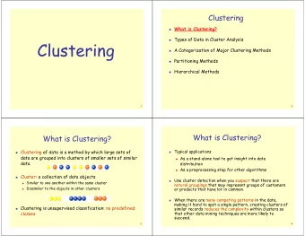
Cluster analysis  Data collected for N samples.  For each sample, measurements made on G variables.  Data represented as a G x N matrix. C5 C6  The objective is to cluster the N samples into a few classes in such a way that C3 samples within a class are collectively more similar to C1 each other than to samples C4 in any other class. C2 2

Cluster analysis methods  There are many standard approaches available (e.g., partitioning methods such as K-means, hierarchical methods such as average linkage, machine learning methods such as self organizing maps)  For example, hierarchical clustering is one of the more popular clustering methods. -- Define an inter-sample dissimilarity (e.g., Euclidean distance, 1-Correlation) -- Define an inter-cluster dissimilarity (e.g., Dissimilarity between a pair of clusters is the average dissimilarity between a sample in one cluster and a sample in the other cluster) -- Combine “close” samples/clusters sequentially 3

Hierarchical clustering: how it works 1 2 3 4 5 6 SAMPLE 2 SAMPLE 3 SAMPLE 4 SAMPLE 5 SAMPLE 6 SAMPLE 7 SAMPLE 1 7 4

The catch  In many contemporary settings, the data are megavariate, i.e., N << G (e.g., in high throughput gene expression studies G is around 1,000-50,000 while N is around 10-500); in such cases, most predictors are noninformative and could overwhelm the dissimilarity estimates.  Example: Use gene expression data to discover unexpected novel classes among the samples (e.g., in leukemia patients, subtypes of leukemia). 5

Case study  Experiment: Compare the gene expression profiles of 6 KO mice vs 6 WT mice using a microarray with 45101 genes. WT: C1 C2 C3 C4 C5 C6 KO: T1 T2 T3 T4 T5 T6  Note 1: Data available for early stage and late stage development of these mice.  Note 2: This data is useful for illustration but is not representative of a cluster analysis situation as here 6 the classes are known.

Gene expression data  Gene expression levels (measured via microarrays) for G genes in N samples: C1 C2 C3 C4 C5 C6 … G1 83 94 82 111 130 122 G2 16 14 7 2 11 33 G3 490 879 193 604 1031 962 G4 46458 49268 74059 44849 42235 44611 G5 32 70 185 20 25 19 G6 1067 891 546 906 1038 1098 G7 118 111 95 896 536 695 G8 10 30 25 24 31 28 G9 166 132 162 27 109 213 G10 136 139 44 62 23 135 . . . . . . . . . . . . . . . . . . . . . . . . Preprocess and analyze 7

Biplots of data from knockout experiment Early stage Late stage 8

Clustering of data from knockout experiment Early stage Late stage MR=5/12 MR=0/12 9

Filtering  Problem: With megavariate data, most predictors are noninformative and will overwhelm the dissimilarity estimates.  Usual (partial) resolution: Filter the genes based on variance or coefficient of variation to reduce the error rates (but which genes are informative?).  Resolution: Ensemble approach: Filter genes repeatedly and apply an ensemble technique. 10

Select n samples and g genes Gene expression matrix S1 S2 S4 S5 S6 S1 S2 S3 S4 S5 S6 G8523 680 749 669 724 643 G8521 1003 1306 713 1628 1268 1629 G8524 262 311 1677 1286 1486 890 705 566 975 883 1005 G8522 G8528 2571 1929 2439 1613 5074 680 749 811 669 724 643 G8523 262 311 336 1677 1286 1486 G8530 1640 1693 1731 1861 1550 G8524 254 383 258 1652 1799 1645 G8525 G8537 4077 2557 3394 2926 2755 81 140 288 298 241 342 G8526 G8545 1652 1799 254 383 258 G8527 4077 2557 2600 3394 2926 2755 G8547 2607 3394 2755 3077 2227 G8528 2571 1929 1406 2439 1613 5074 55 73 121 22 141 44 G8529 Compute similarity G8530 1640 1693 1517 1731 1861 1550 168 229 284 220 310 315 G8531 323 258 359 345 308 315 G8532 Similari ty S1 S2 S3 S4 S5 S6 Similarity S1 S2 S3 S4 S5 S6 Similarity S1 S2 S3 S4 S5 S6 Similarity S1 S2 S3 S4 S5 S6 Similarity S1 S2 S3 S4 S5 S6 Similarity S1 S2 S3 S4 S5 S6 G8533 12131 11199 14859 11544 11352 11506 0 1 1 1 0 0 0 1 0 0 0 0 0 6 7 7 0 0 0 2 3 3 0 0 0 1 1 1 0 0 0 1 2 2 0 0 G8534 11544 11352 12131 11199 14859 12529 S1 S1 S1 S1 S1 S1 G8535 1929 1406 2439 254 383 258 S2 S2 1 0 0 0 1 1 1 0 0 0 0 0 S2 S2 S2 S2 1 0 0 0 0 0 6 0 5 5 1 1 2 0 1 1 1 1 1 0 0 0 1 1 191 140 288 298 241 342 G8536 G8537 4077 2557 2600 3394 2926 2755 S3 S3 1 0 0 2 0 0 0 0 0 0 0 0 S3 S3 S3 S3 1 0 0 1 0 0 7 5 0 8 0 0 2 0 0 3 0 0 3 1 0 4 0 0 G8538 2571 1613 5074 1652 1799 1645 S4 S4 1 0 2 0 1 1 0 0 0 0 1 1 S4 S4 1 0 1 0 1 1 2 0 3 0 1 1 S4 S4 3 1 4 0 1 1 7 5 8 0 2 2 55 73 121 22 91 24 G8539 G8540 1640 1693 1517 1731 1861 1750 S5 0 0 0 1 0 1 S5 S5 S5 0 0 0 1 0 2 0 1 0 1 0 3 0 1 0 1 0 4 S5 0 2 0 2 0 10 S5 0 1 0 1 0 5 168 229 284 220 312 335 G8541 323 258 359 345 298 325 G8542 S6 0 0 0 1 1 0 S6 0 1 0 1 3 0 S6 S6 0 0 0 1 2 0 0 1 0 1 4 0 S6 S6 0 2 0 2 10 0 0 1 0 1 5 0 G8543 2007 1878 1502 1758 2480 1731 G8544 2480 1731 2007 1878 1502 1758 G8545 1652 1799 1645 254 383 258 298 241 342 81 150 298 G8546 Final Clusters G8547 2607 3394 2926 2755 3077 2227 G8548 2571 1929 1406 2439 1613 5074 121 22 55 730 201 35 G8549 G8550 1640 1693 1517 1731 1861 1550 {S1,S2,S3,S4} {S5,S6} 11

ABC dissimilarities Data Simple or weighted Simple random sample of cases based on variance Random sample of genes Cluster analysis HC (Ave, Ward’s), Kmeans, … Iterate ABC(i,j) = 1-relative frequency Input to clustering of how often samples i and j algorithm cluster together 12 Ref: Amaratunga, Cabrera and Kovtun ( Biostatistics , 2007)

ABC clustering of data from knockout experiment Early stage Late stage MR=2/12 MR=0/12 13

ABC-MDS plot of data from knockout experiment Early stage Late stage 14

Within-cluster and between-cluster dissimilarities 15

More proof-of-concept examples  Try on data in which the clusters are known. Misclassification Rates Method Golub AMS ALL Colon 18.1 1.4 0.0 9.7 Ward's with ABC 23.6 9.7 2.3 48.4 Ward’s with 1-Cor Single Linkage 47.0 47.0 25.0 37.0 Complete Linkage 37.5 23.6 41.4 45.0 Average Linkage 47.2 27.8 26.5 38.7 20.8 5.5 42.2 48.4 K-means 23.6 8.3 2.3 16.1 PAM Random Forest 43.0 26.4 48.0 43.5 16

More proof-of-concept examples (ctd)  … with feature selection Misclassification Rates Method Golub AMS ALL Colon 18.1 1.4 0.0 9.7 Ward's with ABC 6.9 13.9 0.0 24.2 Ward’s with 1-Cor Single Linkage 45.8 58.3 26.6 35.5 Complete Linkage 29.2 13.9 0.0 27.4 Average Linkage 5.6 30.6 0.0 37.1 6.9 6.9 0.0 14.5 K-means 8.3 13.9 0.0 12.9 PAM Random Forest 23.6 12.5 0.0 11.3 17

Hepatotoxicity example (1)  In this experiment N=87 compounds were tested in rats for a certain type of hepatotoxicity. 18

Hepatotoxicity example (2)  ABC was run on this dataset. 0.4 Nim Phe ANI Gli Sul Die Flu Cy p Ami Dis Met But Bro Ace Flu Nia Par Tan 0.2 Vit Chl Tam Car Adr Ket Sim Hy d Car Cis Pro Dan Pur Ver Pip Eth Met Fur Phe Met Iso Tes 0.0 Str Sul Tac Dex Ami Ate Ams ChoSpi Iso Dap Sta Ani Dig Val Cad Ery Eto Dic Dox Cy c Bro Dac Met Ral -0.2 Cap Ran Met Bus Fam Asp Ace Rif Per Nal Mif Tet Rot -0.4 Gen Chl Bus Dip Clo Meb Niz My c Met -0.4 -0.2 0.0 0.2 0.4 19

Hepatotoxicity example (3)  In this case, it was known that there are 3 genes thought to be implicated with the toxicity of interest. 20

Hepatotoxicity example (4)  Running ABC with weights proportional to the maximum correlation to these 3 genes gave a much more interesting result. Acet Adre Spir Chol Dich Stan Test Amin Aten Digo Dexa My co Niza Phen Simv Ison Stre Vera Meth Ralo Isop Prog 0.2 Doxo Mif e Mebe Rani Para Metf Daca Meto Gent Cy cl Busp Tetr 0.0 Pipe Meth Ethi Brom Keto Buty Flut Meth Nime Disu Cy pr Phen Dipy Vita ANIT Nalt Acet Tann Famo Tamo Anil Cadm Suli Amsa Busu Chlo Carb Cloz Valp Sulf Diel Glib -0.2 Aspi Hy dr Chlo Carm Niac Dant Daps Fluo Rif a Etop -0.4 Cisp Tacr Puro Capt Furo Brom Rote Meth Perh Ery t Amio -0.2 0.0 0.2 0.4

Extension: ensemble classifiers Data Simple random sample of subjects Simple random sample of genes Tree (  Random Forest*), LDA, … Construct classifier Predict using classifier Prediction: Collate results Majority Vote 22 Ref: Breiman ( Machine Learning , 2001), Amaratunga et al (2009)

Case study: KO experiment  Try on data in which the classes are known. Out-of-bag error rates E- EE- RF RF( p ) ERF LDA LDA Slc17A5 Day 0 0.583 0.583 0.167 0.583 0.083 Slc17A5 Day 18 0.083 0.083 0.000 0.000 0.000 Slc17A5 Day 0 0.750 0.750 0.833 0.833 0.833 (scrambled) Slc17A5 Day 18 0.583 0.667 0.667 0.583 0.583 (scrambled) 23 Ref: Amaratunga, Cabrera & Lee ( Bioinformatics , 2008)