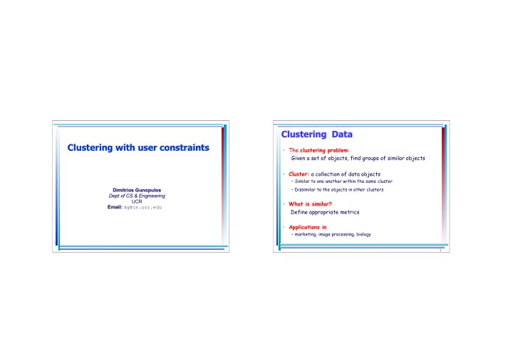
Clustering Data Clustering with user constraints The clustering - PowerPoint PPT Presentation

Clustering Data Clustering with user constraints • The clustering problem : Given a set of objects, find groups of similar objects � • Cluster: a collection of data objects – Similar to one another within the same cluster – Dissimilar to the objects in other clusters Dimitrios Gunopulos Dept of CS & Engineering � UCR • What is similar? Email: dg@cs.ucr.edu Define appropriate metrics � • Applications in – marketing, image processing, biology � 2

Clustering Methods K-Means and K-Medoids algorithms • K-Means and K-medoids algorithms • Minimizes the sum of square distances of points to cluster – PAM, CLARA, CLARANS [Ng and Han, VLDB 1994] representative � • Hierarchical algorithms 2 � E ∑ x m = − K k c x ( ) – CURE [Guha et al, SIGMOD 1998] k k � – BIRCH [Zhang et al, SIGMOD 1996] • Efficient iterative algorithms (O(n)) – CHAMELEON [IEEE Computer, 1999] � • Density based algorithms – DENCLUE [Hinneburg, Keim, KDD 1998] – DBSCAN [Ester et al, KDD 96] � • Subspace Clustering – CLIQUE [Agrawal et al, SIGMOD 1998] – PROCLUS [Agrawal et al, SIGMOD 1999] – ORCLUS: [Aggarwal, and Yu, SIGMOD 2000] – DOC: [Procopiuc, Jones, Agarwal, and Murali, SIGMOD, 2002] � 3 � 4

1. Ask user how many clusters they’d like. (e.g. K=5) Each data point finds out 2. Randomly guess K cluster center which center it’s closest to. locations *based on slides by Padhraic Smyth UC, Irvine *based on slides by Padhraic Smyth UC, Irvine � 5 � 6

� Problems with K-Means type algorithms 1. Redefine each center finding out the set of the points it owns Advantages ▪ Relatively efficient: O(tkn), - where n is the number of objects, k is the - number of clusters, and t is the number of iterations. Normally, k, t << n. Often terminates at a local optimum . - � ▪ Problems – Clusters are approximately spherical – Unable to handle noisy data and outliers – High dimensionality may be a problem – The value of k is an input parameter *based on slides by Padhraic Smyth UC, Irvine � 7 � 8

Spectral Clustering (I) Spectral Clustering methods • Algorithms that cluster points using eigenvectors of matrices • Method #1 derived from the data – Partition using only one eigenvector at a time � – Use procedure recursively • Obtain data representation in the low-dimensional space that can • Example: Image Segmentation be easily clustered • Method #2 � • Variety of methods that use the eigenvectors differently [Ng, Jordan, Weiss. NIPS 2001] – Use k eigenvectors ( k chosen by user) [Belkin, Niyogi, NIPS 2001] – Directly compute k -way partitioning [Dhillon, KDD 2001] – Experimentally it has been seen to be “better” ([Ng, [Bach, Jordan NIPS 2003] Jordan, Weiss. NIPS 2001][Bach, Jordan, NIPS ’03]). [Kamvar, Klein, Manning. IJCAI 2003] [Jin, Ding, Kang, NIPS 2005] � 9 � 10

Hierarchical Clustering Kernel-based k-means clustering 
 (Dhillon et al., 2004) • Two basic approaches: • Data not linearly separable • merging smaller clusters into larger ones (agglomerative) , • Transform data to high-dimensional space using kernel • splitting larger clusters (divisive) – φ a function that maps X to a high dimensional space � • visualize both via “dendograms” • Use the kernel trick to evaluate the dot products: – a kernel function k (x, y) computes φ (x) ⋅ φ (y) ✓ shows nesting structure • cluster kernel similarity matrix using weighted kernel K-Means. ✓ merges or splits = tree nodes • The goal is to minimize the following objective function: Step 1 Step 2 Step 3 Step 4 Step 0 agglomerative a a b k b ( ) 2 k a b c d e J { } ( ) x m ∑ ∑ π = α ϕ − c i i c c 1 = c c 1 x = ∈ π c d e i c d ( ) ∑ x α ϕ d e i i x ∈ π where m = i c e c divisive ∑ α i x ∈ π i c Step 4 Step 3 Step 2 Step 1 Step 0 � 11 � 12

Hierarchical Clustering: Complexity Density-based Algorithms 10 • Clusters are regions of • Quadratic algorithms space which have a high 8 � • Running time can be density of points improved using sampling 5 � • Clusters can have arbitrary [Guha et al, SIGMOD 1998] 3 shapes 0 r using the triangle 0 0 3 5 8 10 inequality (when it holds) Regions of high density *based on slides by Padhraic Smyth UC, Irvine � 13 � 14

Clustering High Dimensional Data Applying Dimensionality Reduction Techniques Dimensionality reduction techniques (such as Singular Value • Fundamental to all clustering techniques is the choice of Decomposition ) can provide a solution by reducing the distance measure between data points; dimensionality of the dataset: � � � 2 q ( ) ( ) D x , x x x ∑ = − � � i j ik jk k 1 = � � • Assumption : All features are equally important ; � • Such approaches fail in high dimensional spaces Drawbacks: • Feature selection (Dy and Brodley, 2000) Dimensionality Reduction • The new dimensions may be difficult to interpret • They don’t improve the clustering in all cases � 15 � 16

Applying Dimensionality Reduction Techniques Subspace clustering • Subspace clustering addresses the problems that arise from high dimensionality of data – It finds clusters in subspaces: subsets of the attributes � • Density based techniques – CLIQUE: Agrawal, Gehrke, Gunopulos, Raghavan (SIGMOD’98) – DOC: Procopiuc, Jones, Agarwal, and Murali, (SIGMOD, 2002) Different dimensions may be relevant to different • Iterative algorithms clusters – PROCLUS: Agrawal, Procopiuc, Wolf, Yu, Park (SIGMOD’99) In General : Clusters may exist in different subspaces, – ORCLUS: Aggarwal, and Yu (SIGMOD 2000). comprised of different combinations of features � 17 � 18

Subspace clustering Locally Adaptive Clustering Each cluster is characterized by different attribute weights • Density based clusters: find dense (Friedman and Meulman 2002, Domeniconi 2004) areas in subspaces • Identifying the right sets of attributes is hard • Assuming a global threshold allows bottom-up algorithms • Constrained monotone search in a lattice space ( w , w ), w w ( w , w ), w w > > 1 x 1 y 1 x 1 y 2 x 2 y 2 y 2 x � 19 � 20

LAC 
 Locally Adaptive Clustering : Example [ C. Domeniconi et al SDM04] • Computing the weights: X : average squared distance along dimension i of points in before local ji S from c transformations j j 1 ( ) 2 X ∑ c x = − ji ji i S x S j ∈ j X e − ji w Exponential weighting scheme = ji X − ∑ e jl l after local Result : transformations A weight vector for each cluster w , w , , w ! 1 2 k � 21 � 22

Convergence of LAC Semi-Supervised Clustering • Clustering is applicable in many real life scenarios The LAC algorithm converges to a local minimum of the – there is typically a large amount of unlabeled data available. error function: k q � ) ∑∑ X • The use of user input is critical for E ( C , W w e − = ji ji – the success of the clustering process j 1 i 1 = = q 2 subject to the constraints ∑ w 1 j – the evaluation of the clustering accuracy. = ∀ ji i 1 = � • User input is given as [ ] [ ] C c c W w w ! ! = = 1 k 1 k – Labeled data – Constraints EM-like convergence : S Hidden variables : assignments of points to centroids ( ) j Learning approaches that use S w ji c , E-step: find the values of given j ji labeled data/constraints + unlabeled data w ji c , ( ) E C , W ji M-step: find that minimize given current S have recently attracted the interest of researchers j estimates . � 23 � 24

Motivating semi-supervised learning a user may want the • points in B and C to Data are correlated. To recognize clusters, a distance function should belong to the same cluster reflect such correlations. � • Different attributes may have different degree of relevance depending on the application / user requirements (a) (b) � � The right ☹ A clustering algorithm does not provide the criterion to be used. clustering may depend on the user’s perspective. � Semi-supervised algorithms: Define clusters taking into account � Fully automatic techniques are • labeled data or constraints very limited in addressing this problem if we have “labels” we will convert them to “constraints” (c) � 25 � 26

Clustering under constraints Defining the constraints • Use constraints to • A set of points X = {x 1 , …, x n } on which sets of must-link(S) and cannot-link constraints(D) have been defined. – learn a distance function � • Points surrounding a pair of must-link/cannot-link • Must-link constraints S: {(x i , x j ) in X }: x i and x j should belong to the same cluster – points should be close to/far from each other � – guide the algorithm to a useful solution • Cannot-link constraints D: {(x i , x j ) in X} : x i and x j cannot belong to the same cluster – • Two points should be in the same/different clusters • Conditional constraints – δ -constraint and ε -constraint � 27 � 28