Choice with multiple alternatives Specification of the deterministic - PowerPoint PPT Presentation
Choice with multiple alternatives Specification of the deterministic part Michel Bierlaire Introduction to choice models Nonlinear specifications: heteroscedasticity Heteroscedasticity Logit is homoscedastic in i.i.d. across both i and
Choice with multiple alternatives Specification of the deterministic part Michel Bierlaire Introduction to choice models
Nonlinear specifications: heteroscedasticity
Heteroscedasticity Logit is homoscedastic ◮ ε in i.i.d. across both i and n . ◮ In particular, they all have the same variance. Motivation ◮ People may have different level of knowledge (e.g. taxi drivers) ◮ Different sources of data
Heteroscedasticity Data ◮ G groups in the population. ◮ Each individual n belongs to exactly one group g . ◮ Characterized by indicators: � 1 if n belongs to g , δ ng = 0 otherwise and � g δ ng = 1, for all n .
Heteroscedasticity Assumption: variance of error terms is different across groups Consider individual n 1 belonging to group 1, and individual n 2 belonging to group 2. = V in 1 + ε in 1 U in 1 U in 2 = V in 2 + ε in 2 and Var( ε in 1 ) � = Var( ε in 2 ) Modeling Without loss of generality: Var( ε in 1 ) = α 2 2 Var( ε in 2 )
Heteroscedasticity Modeling: scale parameters U in 1 = V in 1 + ε in 1 = V in 1 + ε ′ in 1 = + = + ε ′ α 2 U in 2 α 2 V in 2 α 2 ε in 2 α 2 V in 2 in 2 Variance Var( ε ′ in 2 ) = Var( α 2 ε in 2 )
Heteroscedasticity Modeling: scale parameters U in 1 = V in 1 + ε in 1 = V in 1 + ε ′ in 1 = + = + ε ′ α 2 U in 2 α 2 V in 2 α 2 ε in 2 α 2 V in 2 in 2 Variance Var( ε ′ in 2 ) = Var( α 2 ε in 2 ) α 2 = 2 Var( α 2 ε in 2 )
Heteroscedasticity Modeling: scale parameters U in 1 = V in 1 + ε in 1 = V in 1 + ε ′ in 1 = + = + ε ′ α 2 U in 2 α 2 V in 2 α 2 ε in 2 α 2 V in 2 in 2 Variance Var( ε ′ in 2 ) = Var( α 2 ε in 2 ) α 2 = 2 Var( α 2 ε in 2 ) = Var( ε in 1 )
Heteroscedasticity Modeling: scale parameters U in 1 = V in 1 + ε in 1 = V in 1 + ε ′ in 1 = + = + ε ′ α 2 U in 2 α 2 V in 2 α 2 ε in 2 α 2 V in 2 in 2 Variance Var( ε ′ in 2 ) = Var( α 2 ε in 2 ) α 2 = 2 Var( α 2 ε in 2 ) = Var( ε in 1 ) = Var( ε ′ in 1 )
Heteroscedasticity Modeling: scale parameters U in 1 = V in 1 + ε in 1 = V in 1 + ε ′ in 1 = + = + ε ′ α 2 U in 2 α 2 V in 2 α 2 ε in 2 α 2 V in 2 in 2 Variance Var( ε ′ in 2 ) = Var( α 2 ε in 2 ) α 2 = 2 Var( α 2 ε in 2 ) = Var( ε in 1 ) = Var( ε ′ in 1 ) ε ′ in 1 and ε ′ in 2 can be assumed i.i.d.
Heteroscedasticity Modeling: utility function µ n V in + ε in where G � µ n = δ ng α g g =1 and α g , g = 1 , . . . , G are unknown parameters to be estimated from data. Remarks ◮ Even if V in = � j β j x jin is linear-in-parameters, µ n V in = � j µ n β j x jin is not. ◮ Normalization: one α g must be normalized.
Recommend
More recommend
Explore More Topics
Stay informed with curated content and fresh updates.
