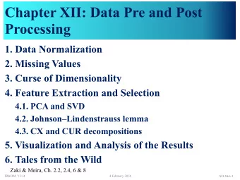
Chapter XII: Data Pre and Post Processing Information Retrieval - PowerPoint PPT Presentation

Chapter XII: Data Pre and Post Processing Information Retrieval & Data Mining Universität des Saarlandes, Saarbrücken Winter Semester 2013/14 XII.1–4- 1

Chapter XII: Data Pre and Post Processing 1. Data Normalization 2. Missing Values 3. Curse of Dimensionality 4. Feature Extraction and Selection 4.1. PCA and SVD 4.2. Johnson–Lindenstrauss lemma 4.3. CX and CUR decompositions 5. Visualization and Analysis of the Results 6. Tales from the Wild Zaki & Meira, Ch. 2.4, 6 & 8 IR&DM ’13/14 30 January 2014 XII.1–4- 2

XII.1: Data Normalization 1. Centering and unit variance 2. Why and why not normalization? IR&DM ’13/14 30 January 2014 XII.1–4- 3

Zero centering • Consider a data D that contains n observations over m variables – n -by- m matrix D • We say D is zero centered if mean ( d i ) = 0 for each column d i of D • We can center any matrix by subtracting from its columns their means IR&DM ’13/14 30 January 2014 XII.1–4- 4

Unit variance and z-scores • Matrix D is said to have unit variance if var ( d i ) = 1 for each column d i of D – The unit variance is obtained by dividing every column with its standard deviation • Data that is zero centered and normalized to unit variance is called the z-scores – Many methods assume the input is z-scores • We can also apply non-linear transformations before normalizing to the z-scores – E.g. taking logarithms (from positive data) or cubic roots (from general data) diminishes the importance of larger values IR&DM ’13/14 30 January 2014 XII.1–4- 5

Why centering? • Consider the red data ellipse – The main direction of variance is from the origin to the data – The second direction is orthogonal to the first – These don’t tell the variance of the data! • If we center the data, the directions are correct IR&DM ’13/14 30 January 2014 XII.1–4- 6

Why unit variance? • Assume one observation is height in meters and other weight in grams – Now weight contains much higher values (for humans, at least) ⇒ weight has more weight in calculations • Division by standard deviation makes all observations equally important – Most values fall between –1 and 1 IR&DM ’13/14 30 January 2014 XII.1–4- 7

When not to center? • Centering cannot be applied to all kinds of data • It destroys non-negativity – E.g. NMF becomes impossible • Centered data won’t contain integers – E.g. counting or binary data – Can hurt interpretability – Itemset mining and BMF become impossible • Centering destroys sparsity – Bad for algorithmic efficiency – We can retain sparsity by only chancing non-zero values IR&DM ’13/14 30 January 2014 XII.1–4- 8

What’s wrong with unit variance? • Dividing by standard deviation is based on the assumption that the values follow Gaussian distribution – Often plausible by the Law of Large Numbers • Not all data is Gaussian – Integer counts • Especially over a small range – Transaction data – … IR&DM ’13/14 30 January 2014 XII.1–4- 9

XII.2: Missing values 1. Handling missing values 2. Imputation IR&DM ’13/14 30 January 2014 XII.1–4- 10

Missing values • Missing values are common in real-world data – Unobserved – Lost in collection – Error in measurement device – … • Data with missing values needs to be dealt with care – Some methods are robust to missing values • E.g. naïve Bayes classifiers – Some methods cannot (natively) handle missing values • E.g. support vector machines IR&DM ’13/14 30 January 2014 XII.1–4- 11

Handling missing values • Two common techniques to handle missing values are – Imputation – Ignoring them • In imputation , the missing values are replaced with “educated guesses” – E.g. the mean value of the variable • Perhaps stratified over some class – The mean height vs. the mean height of the males – Or a model is fitted to the data and the missing values are drawn from the model • E.g. a low-rank matrix factorization that fits the observed values – This technique is used with lots of missing values in matrix completion IR&DM ’13/14 30 January 2014 XII.1–4- 12

Some problems • Imputation might impute wrong values – This might have significant effect on the results – Especially categorical data is hard • The effect of imputation is never “smooth” • Ignoring records or variable with missing values might not be possible – There might not be any data left • Especially binary data has the problem of distinguishing non-existent and non-observed data – E.g. if data says that certain species does not observed in certain area, it does not mean the species couldn’t live there IR&DM ’13/14 30 January 2014 XII.1–4- 13

XII.3: Curse of Dimensionality 1. The Curse 2. Some oddities of high-dimensional spaces IR&DM ’13/14 30 January 2014 XII.1–4- 14

Curse of dimensionality • Many data mining algorithms need to work in high- dimensional data • But life gets harder as dimensionality increases – The volume grows too fast • 100 points evenly-spaced points in unit interval have max distance between adjacent points of 0.01 • To get that distance for adjacent points in 10-dimensional unit hypercube requires 10 20 points • Factor of 10 18 increase • High-dimensional data also makes algorithms slower IR&DM ’13/14 30 January 2014 XII.1–4- 15

Hypersphere and hypercube • Hypercube is d- dimensional cube with edge length 2r – Volume: vol( H d (2 r )) = (2 r ) d • Hypersphere is the d -dimensional ball of radius r – vol(S 1 ( r )) = 2 r – vol(S 2 ( r )) = π r 2 – vol(S 3 ( r )) = 4/3 π r 3 π d/ 2 – vol(S d ( r )) = K d r d , where K d = Γ ( d/ 2 + 1 ) • Γ ( d /2 + 1) = ( d /2)! for even d IR&DM ’13/14 30 January 2014 XII.1–4- 16

Hypersphere within hypercube Mass is in the corners! -r -r r 0 0 r Fraction of volume hypersphere has of surrounding hypercube: π d/ 2 vol ( S d ( r )) vol ( H d ( 2 r )) = lim lim 2 d Γ ( d/ 2 + 1 ) → 0 d → ∞ d → ∞ 2D 3D 4D higher dimensions IR&DM ’13/14 30 January 2014 XII.1–4- 17

Volume of thin shell of hypersphere S d ( r , ε ) r vol( S d ( r , ε )) = vol( S d ( r )) – vol( S d ( r – ε )) = K d r d – K d ( r – ε ) d r − � � vol ( S d ( r , ✏ )) ⌘ d ⇣ 1 − ✏ Fraction of volume in the shell: = 1 − vol ( S d ( r )) r vol ( S d ( r , ✏ )) ⌘ d ⇣ 1 − ✏ = lim lim d → ∞ 1 − → 1 vol ( S d ( r )) r d → ∞ Mass is in the shell! IR&DM ’13/14 30 January 2014 XII.1–4- 18

XII.4: Feature Extraction and Selection 1. Dimensionality reduction and PCA 1.1. PCA 1.2. SVD 2. Johnson–Lindenstrauss lemma 3. CX and CUR decompositions IR&DM ’13/14 30 January 2014 XII.1–4- 19

Dimensionality reduction • Aim: reduce the number of features/dimensions by replacing them with new ones – The new features should capture the “essential part” of the data – What is considered essential defines what method to use – Vice versa, using wrong dimensionality reduction can lead to non-sensical results • Usually dimensionality reduction methods work on numerical data – For categorical or binary data, feature selection can be more appropriate IR&DM ’13/14 30 January 2014 XII.1–4- 20

Principal component analysis • The goal of the principal component analysis (PCA) is to project the data onto linearly uncorrelated variables in (possibly) lower-dimensional subspace that preserves as much of the variance of the original data as possible – Also known as Karhunen–Lòeve transform or Hotelling transform • And with many other names, too • In matrix terms, we want to find a column-orthogonal n -by- r matrix U that projects n -dimensional data vector x into r -dimensional vector a = U T x IR&DM ’13/14 30 January 2014 XII.1–4- 21

Deriving the PCA: 1-D case (1) • We assume our data is normalized to z-scores • We want to find a unit vector u that maximizes the variance of the projections u T x i u – Scalar u T x i gives the coordinate of x i along u – As data is normalized, its mean is 0, which has coordinate 0 when projected to u • The variance of the projection is n n Σ = 1 σ 2 = 1 X X ( u T x i − µ u ) 2 x i x T i n n i = 1 i = 1 = u T Σ u The covariance matrix for centered data IR&DM ’13/14 30 January 2014 XII.1–4- 22

Deriving the PCA: 1-D case (2) • To maximize variance σ 2 , we maximize J ( u ) = u T Σ u − λ ( u T u − 1 ) – The second term is to ensure u is a unit vector • Solving the derivative gives Σ u = λ u – u is an eigenvector and λ is an eigenvalue – Further u T Σ u = u T λ u implying that σ 2 = λ • To maximize variance, we need to take the largest eigenvalue • Thus, the first principal component u is the dominant eigenvector of the covariance matrix Σ IR&DM ’13/14 30 January 2014 XII.1–4- 23

Example of 1-D PCA X 3 X 1 X 2 u 1 Figure 7.2: Best One-dimensional or Line Approximation IR&DM ’13/14 30 January 2014 XII.1–4- 24