Chapter VIII: Clustering Information Retrieval & Data Mining - PowerPoint PPT Presentation
Chapter VIII: Clustering Information Retrieval & Data Mining Universitt des Saarlandes, Saarbrcken Winter Semester 2013/14 VIII.1&2- 1 Chapter VIII: Clustering* 1. Basic idea 2. Representative-based clustering 2.1. k -means
Chapter VIII: Clustering Information Retrieval & Data Mining Universität des Saarlandes, Saarbrücken Winter Semester 2013/14 VIII.1&2- 1
Chapter VIII: Clustering* 1. Basic idea 2. Representative-based clustering 2.1. k -means 2.2. EM-clustering 3. Hierarchical clustering 3.1. Basic idea 3.2. Cluster distances 4. Density-based clustering 5. Co-clustering 6. Discussion and clustering applications *Zaki & Meira, Chapters 13–15; Tan, Steinbach & Kumar, Chapter 8 IR&DM ’13/14 7 January 2014 VIII.1&2- 2
1. Basic idea 1. Example 2. Distances between objects IR&DM ’13/14 7 January 2014 VIII.1&2- 3
Example Low inter-cluster similarity High intra-cluster similarity An outlier? IR&DM ’13/14 7 January 2014 VIII.1&2- 4
The clustering task • Given a set U of objects and a distance d : U 2 → R + between them, group objects of U into clusters such that the distance between points in the same cluster is low and the distance between the points in different clusters is large – Small and large are not well defined – Clustering can be • exclusive (each point belongs to exactly one cluster) • probabilistic (each point-cluster pair is associated with a probability of the point belonging to that cluster) • fuzzy (each point can belong to multiple clusters) – Number of clusters can be pre-defined or not IR&DM ’13/14 7 January 2014 VIII.1&2- 5
On distances • A function d : U 2 → R + is a metric if: – d ( u , v ) = 0 if and only if u = v Self-similarity – d ( u , v ) = d ( v , u ) for all u , v ∈ U Symmetry Triangle – d ( u , v ) ≤ d ( u , w ) + d ( w , v ) for all u , v , and w ∈ U inequality • A metric is a distance ; if d : U 2 → [0, a ] for some positive a , then a – d ( u , v ) is similarity • Common metrics: i = 1 | u i − v i | p ⌘ 1 ⇣ P d – L p : for d -dimensional space p • L 1 = Hamming = city-block; L 2 = Euclidean – Correlation distance: 1 – φ – Jaccard distance: 1 – | A ∩ B | / | A ∪ B | IR&DM ’13/14 7 January 2014 VIII.1&2- 6
More on distances • For all-numerical data, the sum of squared errors (SSE) is the most common one P d – SSE: i = 1 | u i − v i | 2 • For all-binary data, either Hamming or Jaccard is used • For categorical data either – first convert the data to binary by adding one binary variable per category label and then use Hamming; or – count the agreements and disagreements of category labels with Jaccard • For mixed data, some combination must be used IR&DM ’13/14 7 January 2014 VIII.1&2- 7
Implicit distance and distance matrix d 1,2 d 1,3 d 1, n 0 d 1,2 0 d 2,3 d 2, n · · · d 1,3 d 2,3 d 3, n 0 . . ... . . . . d 1, n d 2, n d 3, n 0 · · · A distance (or dissimilarity ) matrix is • n -by- n for n objects • non-negative ( d i,j ≥ 0) • symmetric ( d i,j = d j,i ) • zero on diagonal ( d i,i = 0) IR&DM ’13/14 7 January 2014 VIII.1&2- 8
2. Representative-based clustering 1. Partitions and prototypes 2. The k -means algorithm 2.1. Basic algorithm 2.2. Analysis 2.3. The k -means++ algorithm 3. The EM clustering algorithm 3.1. 1-D Gaussian 3.2. General Gaussian 3.3. The k -means as EM 4. How to select the k IR&DM ’13/14 7 January 2014 VIII.1&2- 9
Partitions and prototypes • Exclusive representative-based clustering: – The set of objects U is partitioned into k clusters C 1 , C 2 , ..., C k • ∪ i C i = U and C i ∩ C j = ∅ for i ≠ j – Each cluster is represented by a prototype (also called centroid or mean) µ i • Prototype does not have to be (and usually is not) one of the objects Over all objects in this cluster – Clustering quality is based on sum of squared errors between objects in cluster and cluster prototype k k d X X k x j − µ i k 2 X X X ( x jl − µ il ) 2 2 = i = 1 x j ∈ C i i = 1 x j ∈ C i l = 1 Over all dimensions Over all clusters IR&DM ’13/14 7 January 2014 VIII.1&2- 10
The naïve algorithm • The naïve algorithm: – Generate all possible clusterings one-by-one – Compute the squared error – Select the best • But this approach is infeasible – There are too many possible clusterings to try • k n different clusterings to k clusters (some possibly empty) • The number of ways to cluster n points in k nonempty clusters is the Stirling number of the second kind, S ( n , k ), k � n � ✓ k ◆ = 1 X ( − 1 ) j ( k − j ) n S ( n , k ) = k k ! j j = 0 IR&DM ’13/14 7 January 2014 VIII.1&2- 11
An iterative k -means algorithm 1. select k random cluster centroids 2. assign each point to its closest centroid and compute the error 3. do 3.1. for each cluster C i 3.1.1. compute new centroid as 1 P µ i = x j ∈ C i x j | C i | 3.2. for each element x j ∈ U 3.2.1. assign x j to its closest cluster centroid 4. while error decreases IR&DM ’13/14 7 January 2014 VIII.1&2- 12
k -means example 5 5 5 5 5 4 4 4 4 k 1 k 1 k 1 k 1 4 k 1 expression in condition 2 3 3 3 3 k 2 k 2 3 2 2 2 2 k 3 k 3 k 2 1 k 3 k 2 k 2 1 1 1 1 k 3 k 3 0 0 0 0 0 1 2 3 4 5 0 0 0 1 1 1 2 2 2 3 3 3 4 4 4 5 5 5 0 0 1 3 4 5 expression in condition 1 IR&DM ’13/14 7 January 2014 VIII.1&2- 13
Some notes on the algorithm • Always converges eventually – On each step the error decreases – Only finite number of possible clusterings – Convergence to local optimum • At some point a cluster can become empty – All points are closer to some other centroid – Some options: • Split the biggest cluster • Take the furthest point as a singleton cluster • Outliers can yield bad clusterings IR&DM ’13/14 7 January 2014 VIII.1&2- 14
Computational complexity • How long does the iterative k -means algorithm take? – Computing the centroid takes O( nd ) time • Averages over total of n points in d -dimensional space – Computing the cluster assignment takes O( nkd ) time • For each n points we have to compute the distance to all k clusters in d -dimensional space – If the algorithm takes t iterations, the total running time is O( tnkd ) – But how many iterations we need? IR&DM ’13/14 7 January 2014 VIII.1&2- 15
How many iterations? • In practice the algorithm doesn’t usually take many iterations – Some hundred iterations is usually enough • Worst-case upper bound is O( n dk ) • Worst-case lower bound is superpolynomial: 2 Ω ( √ n ) • The discrepancy between practice and worst-case analysis can be (somewhat) explained with smoothed analysis [Arthur & Vassilvitskii ’06]: – If the data is sampled from independent d -dimensional normal distributions with same variance, iterative k -means algorithm will terminate in time O( n k ) with high probability. IR&DM ’13/14 7 January 2014 VIII.1&2- 16
On the importance of initial centroids Iteration 1 Iteration 2 Iteration 3 Iteration 1 Iteration 2 3 3 3 3 3 2.5 2.5 2.5 2.5 2.5 2 2 2 2 2 1.5 1.5 1.5 1.5 1.5 y y y y y 1 1 1 1 1 0.5 0.5 0.5 0.5 0.5 0 0 0 0 0 The k-means algorithm converges to local optimum -2 -1.5 -1 -0.5 0 0.5 1 1.5 2 -2 -1.5 -1 -0.5 0 0.5 1 1.5 2 -2 -1.5 -1 -0.5 0 0.5 1 1.5 2 -2 -1.5 -1 -0.5 0 0.5 1 1.5 2 -2 -1.5 -1 -0.5 0 0.5 1 1.5 2 x x x x x which can be arbitrary bad vs. the global optimum. Iteration 3 Iteration 4 Iteration 5 Iteration 4 Iteration 5 Iteration 6 3 3 3 3 3 3 2.5 2.5 2.5 2.5 2.5 2.5 2 2 2 2 2 2 1.5 1.5 1.5 1.5 1.5 1.5 y y y y y y 1 1 1 1 1 1 0.5 0.5 0.5 0.5 0.5 0.5 0 0 0 0 0 0 -2 -1.5 -1 -0.5 0 0.5 1 1.5 2 -2 -1.5 -1 -0.5 0 0.5 1 1.5 2 -2 -1.5 -1 -0.5 0 0.5 1 1.5 2 x x x -2 -1.5 -1 -0.5 0 0.5 1 1.5 2 -2 -1.5 -1 -0.5 0 0.5 1 1.5 2 -2 -1.5 -1 -0.5 0 0.5 1 1.5 2 x x x IR&DM ’13/14 7 January 2014 VIII.1&2- 17
The k-means++ algorithm • Careful initial seeding [Arthur & Vassilvitskii ’07]: – Choose first centroid u.a.r. from data points – Let D ( x ) be the shortest distance from x to any already-selected centroid D ( x 0 ) 2 – Choose next centroid to be x’ with probability P x 2 X D ( x ) 2 • Points that are further away are selected more probably – Repeat until k centroids have been selected and continue as normal iterative k -means algorithm • The k -means++ algorithm achieves O (log k ) approximation ratio on expectation – E [cost] ≤ 8(ln k + 2)OPT • The k -means++ algorithm converges fast in practice IR&DM ’13/14 7 January 2014 VIII.1&2- 18
Limitations of cluster types for k-means • The clusters have to be of roughly equal size • The clusters have to be of roughly equal density • The clusters have to be of roughly spherical shape K-means (3 Clusters) K-means (3 Clusters) Original Points Original Points Original Points K-means (2 Clusters) IR&DM ’13/14 7 January 2014 VIII.1&2- 19
Recommend
More recommend
Explore More Topics
Stay informed with curated content and fresh updates.
