Chapter 7: Sampling In this chapter we will cover: 1. Samples and - PDF document

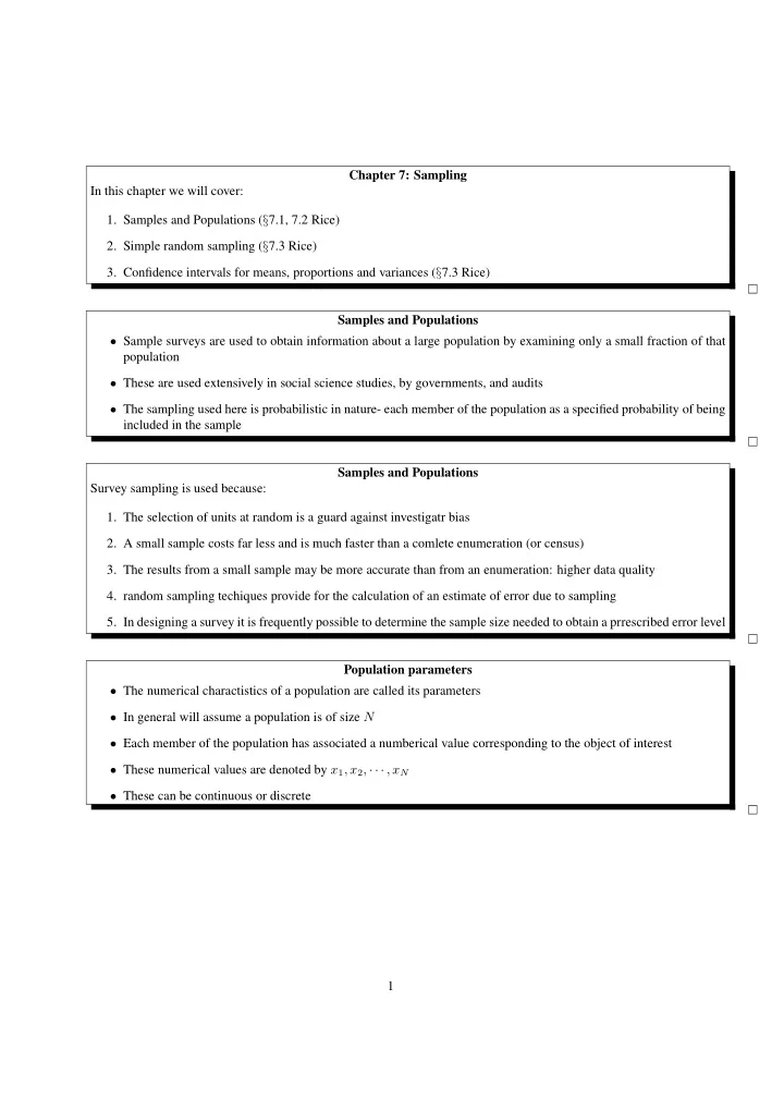
Chapter 7: Sampling In this chapter we will cover: 1. Samples and Populations ( § 7.1, 7.2 Rice) 2. Simple random sampling ( § 7.3 Rice) 3. Confidence intervals for means, proportions and variances ( § 7.3 Rice) Samples and Populations • Sample surveys are used to obtain information about a large population by examining only a small fraction of that population • These are used extensively in social science studies, by governments, and audits • The sampling used here is probabilistic in nature- each member of the population as a specified probability of being included in the sample Samples and Populations Survey sampling is used because: 1. The selection of units at random is a guard against investigatr bias 2. A small sample costs far less and is much faster than a comlete enumeration (or census) 3. The results from a small sample may be more accurate than from an enumeration: higher data quality 4. random sampling techiques provide for the calculation of an estimate of error due to sampling 5. In designing a survey it is frequently possible to determine the sample size needed to obtain a prrescribed error level Population parameters • The numerical charactistics of a population are called its parameters • In general will assume a population is of size N • Each member of the population has associated a numberical value corresponding to the object of interest • These numerical values are denoted by x 1 , x 2 , · · · , x N • These can be continuous or discrete 1

Example A • The population is N = 393 short stay hospitals • The data is x i which is the number of patients discharged from the i th hospital in Januray 1968 • The population mean is N µ = 1 � x i , N i =1 this is 814.6 • The population total is N � τ = x i = Nµ, i =1 this is 320 138 • population variance is N σ 2 = 1 � ( x i − µ ) 2 N i =1 Example A Number of discharges 70 60 50 40 Frequency 30 20 10 0 0 500 1000 1500 2000 2500 3000 Number of discharges 2

Simple random sampling • The most elementary form of sampling is simple random sampling (s.r.s.) • Here each sample of size n has the same probability of being selected � N � • The sampling is done without replacement so there are possible samples n Sample mean • If the sample size is n then denote the sample by X 1 , X 2 , · · · , X n • Each is a random variable • The sample mean is then n X = 1 ¯ � X i n i =1 • This is also a random variable and will have a (sampling) distribution • We will use ¯ X which is calculated from the sample to estimate µ , which can only be calculated from the population • In practice we will know the sample but not know the population Example A • We would like to know the sampling distrubution of barX for each n • If n = 16 there are 10 33 different samples, so we cann’t enumerate exactly the sampling distrubition • We can simulate it though, i.e. draw the sample many (500-1000) times and examine the distribution. • In practice use the fact that the sampling distribution is approximately Normal 3

Example A Sampling dist: n=8 Sampling dist: n=16 140 100 100 80 Frequency Frequency 60 60 40 20 20 0 0 500 1000 1500 500 1000 1500 sample mean sample mean Sampling dist: n=32 Sampling dist: n=64 150 80 100 60 Frequency Frequency 40 50 20 0 0 500 1000 1500 500 1000 1500 sample mean sample mean Example A • All the sampling distributions are centered near the true value, (the red line) • As the sample size increases the histogram becomes less spread out i.e. variance decreases • For the larger values of n the histograms look well approximated by Normal distributions 4

Simple random sampling The following results are proved in Rice (pp. 191-194) • For simple random sampling E ( ¯ X ) = µ We say ¯ X is an unbiased estimate of µ • For simple random sampling E ( T ) = τ We say T is an unbiased estimate of τ • For simple random sampling X ) = σ 2 � 1 − n − 1 � V ar ( ¯ n N − 1 The term n − 1 N − 1 is called the finite population correction. If N is much bigger than n this will be small Mean square error • An unbiased estimate of a parameter is correct ‘on average’ • One of measuring how good an estimate ˆ θ is of the parameter θ is by using the mean squared error �� � 2 � ˆ mse = E θ − θ • We can rewrite the mse as mse = variance + bias 2 Standard error • Since ¯ X is unbiased its mse is just its variance • As long as n << N this is well approximated by X ) = σ 2 ≈ σ 2 � 1 − n − 1 � V ar ( ¯ n N − 1 n • The term �� σ 1 − n − 1 � σ √ n √ n σ ¯ X = ≈ N − 1 is called the standard error for ¯ X . It measures how close the estimate is to the true value on average • As n gets bigger the standard error gets smaller 5

Estimating a proportion • Suppose the population was split into two groups, one group with some property and another group without • Let the proportion with the property be p • An estimate for p is ˆ p which is the proportion in the sample with the property • This estimate is also unbiased • Its standard error is � � � p (1 − p ) 1 − n − 1 p (1 − p ) σ ˆ p = N − 1 ≈ n n Estimating a population variance • By taking a random sample the population variance σ 2 can be estimated by the variance of the sample n σ 2 = 1 � ( X i − ¯ X ) 2 ˆ n i =1 • This is in fact a biased estimate since � n − 1 � � N � σ 2 ) = σ 2 E (ˆ n N − 1 • An unbiased estimate of V ar ( ¯ X ) is X = s 2 1 − n � � s 2 ¯ n N where n 1 s 2 = � ( X i − ¯ X ) 2 n − 1 i =1 Example A • A simple random sample of 50 of the 393 hospitals was taken. From this sample ¯ X = 938 . 5 • The sample variance is s 2 = 614 . 53 2 • The estimated standard error of ¯ X is X = s 2 1 − n � � s 2 = 81 . 19 ¯ n N Recommended Questions From Rice § 7.7 please look at Questions 1, 3, 5, 6, 7 6

The Normal approximation to sampling distributions • We have calculate the mean and standard deviation of ¯ X , can we find the sampling distribution? • In general the exact sampling distribution will depend on the population distribution which is unknown • The central limit theorem however tells us that we can get a good approximation if n the sample size is large enough The Normal approximation to sampling distributions • The central limit theorem states that if X i are independent with the same distribution then � ¯ X n − µ � P σ/ √ n ≤ z → Φ( z ) , as n → ∞ where µ, σ are the mean and standard deviation of each X i and Φ is the cdf for the standard normal • For simple random sampling the random variables are not strictly independent, nevertheless for n/N sufficiently small a form of the CLT still applies Example A • For the 393 hospitals the standard error for ¯ X when n = 64 is � σ 1 − n − 1 σ ¯ X = √ n N − 1 = 67 . 5 • Applying the CLT means we can ask what is the probability that the estimate ¯ X is more than 100 from the true value i.e. want P ( | ¯ X − µ | > 100) = 2 P ( ¯ X − µ > 100) P ( ¯ 1 − P ( ¯ X − µ > 100) = X − µ > 100) � ¯ X − µ > 100 � = 1 − P σ ¯ σ ¯ X X � 100 � ≈ 1 − Φ 67 . 5 = 0 . 069 7

Example A: simulation In the simulation the proportion of samples further than 100 from the true value is 15 . 6% incomparision to the 14% predicted by theory Sampling dist: n=64 + 140 + 1000 + + + + + + 120 + + + + + + + + + + + + + + + + + + + + + + + + + + + + + + 100 900 Frequency 80 Sample 800 60 40 + + + + ++ + + + + + + + 700 + + + + + + + + + + + + + + + + + + 20 + + + + + + + + + 0 600 600 700 800 900 1000 0 100 200 300 400 500 sample mean index The normal approximation also seems reasonable Confidence intervals • The previous example is a good way to understand a confidence interval • A confidence interval for a population parameter θ is a random interval (i.e. an interval that depends on the sample) • It contains the true value some fixed proportion of the times a sample is drawn • A 95% confidence interval contains θ for 95% of the samples • Confidence interval with coverage 1 − α contains the true value 100(1 − α )% times you use it. 8

Confidence intervals 100 95% Confidence intervals 1200 1000 Mean 800 600 400 0 20 40 60 80 100 Index Confidence intervals: Algorithm • If you want to compute a 95% confidence interval from data X 1 , X 2 , · · · , X n using the normal approximation X and s 2 the sample mean and variance of the data • Calculate ¯ X the s.e. of the estimate, this is s/ √ n • Calculate σ ¯ • In Table 2, Appendix B find the z p such that P ( | z | > z p ) = 0 . 05 . This will be z p = 1 . 96 • The confidence interval is � ¯ X , ¯ � X − 1 . 96 σ ¯ X + 1 . 96 σ ¯ X Example X = 1 . 2 and s 2 = 0 . 09 . Suppose that from a sample of size 100 we have ¯ 1. What is the 95% confidence interval for µ ? 2. What is the 99% confidence interval for µ ? 9