Chapter 5 Singular value decomposition and principal component - PDF document

5. Singular value decomposition and principal component analysis 1 Chapter 5 Singular value decomposition and principal component analysis In A Practical Approach to Microarray Data Analysis (D.P. Berrar, W. Dubitzky, M. Granzow, eds.) Kluwer: Norwell, MA, 2003. pp. 91-109. LANL LA-UR-02-4001 Michael E. Wall 1,2 , Andreas Rechtsteiner 1,3 , Luis M. Rocha 1 , 1 Computer and Computational Sciences Division and 2 Bioscience Division, Mail Stop B256, Los Alamos National Laboratory, Los Alamos, New Mexico, 87545 USA, e-mail: {mewall, rocha}@lanl.gov 3 Systems Science Ph.D. Program, Portland State University, Post Office Box 751, Portland, Oregon 97207 USA, e-mail: andreas@sysc.pdx.edu Abstract: This chapter describes gene expression analysis by Singular Value Decomposition (SVD), emphasizing initial characterization of the data. We describe SVD methods for visualization of gene expression data, representation of the data using a smaller number of variables, and detection of patterns in noisy gene expression data. In addition, we describe the precise relation between SVD analysis and Principal Component Analysis (PCA) when PCA is calculated using the covariance matrix, enabling our descriptions to apply equally well to either method. Our aim is to provide definitions, interpretations, examples, and references that will serve as resources for understanding and extending the application of SVD and PCA to gene expression analysis. 1. INTRODUCTION One of the challenges of bioinformatics is to develop effective ways to analyze global gene expression data. A rigorous approach to gene expression analysis must involve an up-front characterization of the structure of the data. In addition to a broader utility in analysis methods, singular value decomposition (SVD) and principal component analysis (PCA) can be valuable tools in obtaining such a characterization. SVD and PCA are common techniques for analysis of multivariate data, and gene expression data are well suited to analysis using SVD/PCA. A single microarray 1 experiment can generate measurements for thousands, or even tens of thousands of genes. Present experiments typically consist of less than ten assays, but can consist of hundreds (Hughes et al. , 2000). Gene expression data are currently rather noisy, and SVD can detect and extract small signals from noisy data. The goal of this chapter is to provide precise explanations of the use of SVD and PCA for gene expression analysis, illustrating methods using simple examples. We describe SVD methods for visualization of gene expression data, representation of the data using a smaller number of variables, and detection of patterns in noisy gene expression data. In addition, we describe the 1

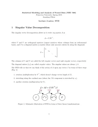
2 Chapter 5 mathematical relation between SVD analysis and Principal Component Analysis (PCA) when PCA is calculated using the covariance matrix, enabling our descriptions to apply equally well to either method. Our aims are 1) to provide descriptions and examples of the application of SVD methods and interpretation of their results; 2) to establish a foundation for understanding previous applications of SVD to gene expression analysis; and 3) to provide interpretations and references to related work that may inspire new advances. In section 1, the SVD is defined, with associations to other methods described. A summary of previous applications is presented in order to suggest directions for SVD analysis of gene expression data. In section 2 we discuss applications of SVD to gene expression analysis, including specific methods for SVD-based visualization of gene expression data, and use of SVD in detection of weak expression patterns. Some examples are given of previous applications of SVD to analysis of gene expression data. Our discussion in section 3 gives some general advice on the use of SVD analysis on gene expression data, and includes references to specific published SVD-based methods for gene expression analysis. Finally, in section 4, we provide information on some available resources and further reading. Mathematical definition of the SVD 2 1.1 Let X denote an m × n matrix of real-valued data and rank 3 r , where without loss of generality m ≥ n , and therefore r ≤ n. In the case of microarray data, x ij is the expression level of the i th gene in the j th assay. The elements of the i th row of X form the n -dimensional vector g i , which we refer to as the transcriptional response of the i th gene. Alternatively, the elements of the j th column of X form the m -dimensional vector a j , which we refer to as the expression profile of the j th assay. The equation for singular value decomposition of X is the following: T X = USV , (5.1) where U is an m × n matrix, S is an n × n diagonal matrix, and V T is also an n × n matrix. The columns of U are called the left singular vectors , { u k }, and form an orthonormal basis for the assay expression profiles, so that u i · u j = 1 for i = j , and u i · u j = 0 otherwise. The rows of V T contain the elements of the right singular vectors , { v k }, and form an orthonormal basis for the gene transcriptional responses. The elements of S are only nonzero on the diagonal, and are called the singular values . Thus, S = diag( s 1 ,..., s n ). Furthermore, s k > 0 for 1 ≤ k ≤ r , and s i = 0 for ( r +1) ≤ k ≤ n . By convention, the ordering of the singular vectors is determined by high-to-low sorting of singular values, with the highest singular value in the upper left index of the S matrix. Note that for a square, symmetric matrix X , singular value decomposition is equivalent to diagonalization, or solution of the eigenvalue problem. One important result of the SVD of X is that ( ) ∑ l l T = X u s v (5.2) k k k = k 1 is the closest rank- l matrix to X . The term “closest” means that X ( l ) minimizes the sum of the squares of the difference of the elements of X and X ( l ) , ∑ ij | x ij – x ( l ) ij | 2 . One way to calculate the SVD is to first calculate V T and S by diagonalizing X T X :

5. Singular value decomposition and principal component analysis 3 T = 2 T X X VS V , (5.3) and then to calculate U as follows: − = XVS 1 U , (5.4) where the ( r +1),..., n columns of V for which s k = 0 are ignored in the matrix multiplication of Equation 5.4. Choices for the remaining n - r singular vectors in V or U may be calculated using the Gram-Schmidt orthogonalization process or some other extension method. In practice there are several methods for calculating the SVD that are of higher accuracy and speed. Section 4 lists some references on the mathematics and computation of SVD. Relation to principal component analysis . There is a direct relation between PCA and SVD in the case where principal components are calculated from the covariance matrix 4 . If one conditions the data matrix X by centering 5 each column, then X T X = Σ i g i g i T is proportional to the covariance matrix of the variables of g i ( i.e. , the covariance matrix of the assays 6 ). By Equation 5.3, diagonalization of X T X yields V T , which also yields the principal components of { g i }. So, the right singular vectors { v k } are the same as the principal components of { g i }. The eigenvalues of X T X are equivalent to s k 2 , which are proportional to the variances of the principal components. The matrix US then contains the principal component scores , which are the coordinates of the genes in the space of principal components. If instead each row of X is centered, XX T = Σ j a j a j T is proportional to the covariance matrix of the variables of a j ( i.e. the covariance matrix of the genes 7 ). In this case, the left singular vectors 2 are again proportional to the { u k } are the same as the principal components of { a j }. The s k variances of the principal components. The matrix SV T again contains the principal component scores, which are the coordinates of the assays in the space of principal components. Relation to Fourier analysis . Application of SVD in data analysis has similarities to Fourier analysis. As is the case with SVD, Fourier analysis involves expansion of the original data in an orthogonal basis: ∑ 2 π = i jk / m x c e (5.5) ij ik k The connection with SVD can be explicitly illustrated by normalizing 8 the vector { e i 2 π jk/m } and by naming it v ' k : ∑ ∑ = = x b v ' u ' s ' v ' (5.6) ij ik jk ik k jk k k which generates the matrix equation X = U ' S ' V ' T , similar to Equation 5.1. Unlike the SVD, however, even though the { v ' k } are an orthonormal basis, the { u ' k } are not in general orthogonal. Nevertheless this demonstrates how the SVD is similar to a Fourier transform, where the vectors { v k } are determined in a very specific way from the data using Equation 5.1, rather than being given at the outset as for the Fourier transform. Similar to low-pass filtering in Fourier analysis, later we will describe how SVD analysis permits filtering by concentrating on those singular vectors that have the highest singular values. 3