Chapter 4 State Feedback LQR Motivation Quadratic minimization : - PDF document

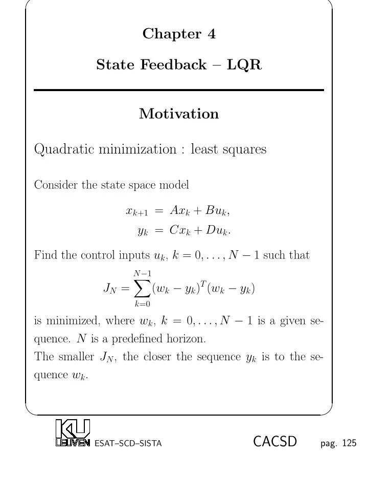
✬ ✩ Chapter 4 State Feedback – LQR Motivation Quadratic minimization : least squares Consider the state space model x k +1 = Ax k + Bu k , y k = Cx k + Du k . Find the control inputs u k , k = 0 , . . . , N − 1 such that N − 1 � ( w k − y k ) T ( w k − y k ) J N = k =0 is minimized, where w k , k = 0 , . . . , N − 1 is a given se- quence. N is a predefined horizon. The smaller J N , the closer the sequence y k is to the se- quence w k . ✫ ✪ CACSD pag. 125 ESAT–SCD–SISTA

✬ ✩ The solution can be derived in terms of the following input-output equations :   H 0 0 · · · · · · 0       y 0 C u 0   H 1 H 0 · · · · · · 0           y 1 CA u 1       = x 0 +   H 2 H 1 H 0 · · · 0       . . .   . . .       . . .         · · · · · · · · · · · · · · ·   CA N − 1 y N − 1   u N − 1 H N − 1 H N − 2 · · · · · · H 0 � �� � � �� � � �� � y u O N � �� � H N where H k are called the Markov parameters (impulse re- sponse matrices) defined as : H 0 = D, H k = CA k − 1 B, k = 1 , 2 , · · · , N − 1 . Let vector w be defined in a similar way as y , then J N = w T w + x T 0 O T N O N x 0 + u T H T N H N u − 2 w T O N x 0 − 2 w T H N u + 2 x T 0 O T N H N u is the quadratic criterion to be minimized. Now find the optimal u as the solution to min u J N . In order to do so we set the derivatives of J N with respect to the vector u to zero, resulting in : H T N H N u = H T N w − H T N O N x 0 . ✫ ✪ CACSD pag. 126 ESAT–SCD–SISTA

✬ ✩ When H T N H N is invertible, then u opt = ( H T N H N ) − 1 H T N ( w − O N x 0 ) , which can be written as         u 0 F 0 G 11 G 12 · · · G 1 N w 0         u 1 F 1 G 21 G 22 · · · G 2 N w 1          =  x 0 +  . . . .         . . . . . · · · · · · · · · · · · .      u N − 1 F N − 1 G N 1 G N 2 · · · G NN w N − 1 Constrained minimization : basics of MPC The least squares solution can be complemented with lin- ear constraints, for instance on the magnitude of the in- put sequence or on its derivative. This then leads to a quadratic programming problem (see Matlab quadprog.m ). One could require for instance that all components of the input u are smaller in absolute value than a certain pre- specified threshold or that they have to be nonnegative (to avoid that too large or too small inputs are applied to the actuators), that the first derivative of the input u stays within certain bounds (to avoid abrupt changes in the in- put), etc ... . ✫ ✪ CACSD pag. 127 ESAT–SCD–SISTA

✬ ✩ Example : Consider the following SISO system       0 . 7 0 . 5 0 1 0 . 1       x k +1 = − 0 . 5 0 . 7 0  x k + 1  u k , x 0 = 0 . 2     0 0 0 . 9 1 0 . 3 � � y k = x k + 0 . 5 u k . 0 − 1 1 We want the output to be as close as possible to a prede- fined w by minimizing ( w − y ) T ( w − y ), where w looks like ( N =20) : desired output w 1 0.8 0.6 0.4 0.2 amplitude 0 −0.2 −0.4 −0.6 −0.8 −1 0 2 4 6 8 10 12 14 16 18 20 discrete time Construct H N and O N . Now compute u as the least squares solution to min u ( w − y ) T ( w − y ) (formula on top of page 127). ✫ ✪ CACSD pag. 128 ESAT–SCD–SISTA

✬ ✩ The input u is shown in the figure below. least squares input u 1000 500 0 −500 amplitude −1000 −1500 −2000 −2500 0 2 4 6 8 10 12 14 16 18 20 discrete time It appears that if this input is applied to the system the output is exactly the desired block wave we wanted. The input however may be too large. Now let’s assume that for safety reasons the input should stay between -100 and 100. Then we have to solve a constrained optimization problem minimizing ( w − y ) T ( w − y ) with respect to u and subject to − 100 ≤ u k ≤ 100. This comes down to a quadratic programming problem which basically solves 1 2 u T Hu + f T u min subject to Au ≤ b. u Matlab program quadprog.m can be used to solve this equation. ✫ ✪ CACSD pag. 129 ESAT–SCD–SISTA

✬ ✩ H and f follow from the expression for J N on page 126 and A and b depend on the constraints which are being applied. The input is shown in the next figure constrained input u 100 80 60 40 20 amplitude 0 −20 −40 −60 −80 −100 0 2 4 6 8 10 12 14 16 18 20 discrete time and clearly remains between the predefined bounds. The output follows the block wave quite well : output y and desired output w 1 0.8 0.6 0.4 0.2 amplitude 0 −0.2 −0.4 −0.6 −0.8 −1 0 2 4 6 8 10 12 14 16 18 20 ✫ ✪ discrete time CACSD pag. 130 ESAT–SCD–SISTA

✬ ✩ A more general quadratic criterion is one in which the in- puts and the outputs are weighted with two weighting ma- trices R ∈ R mN × mN and Q ∈ R pN × pN such that J N = u T Ru + ( y − w ) T Q ( y − w ) . In this way the controller can be better adjusted to the de- signer’s wishes. Furthermore, it appears that this approach is numerically more robust. Try to express J N as a function of w , u , x 0 , ... as on page 126. The optimal solution is now given by u J N = ( R + H T N Q H N ) − 1 ( H T N Qw −H T u opt = min N Q O N x 0 ) . Also in this case the minimization criterion can be comple- mented with linear constraints. The problem with the controller so far is that the input sequences are not really generated by state feedback. If the system model differs from the real system due to inaccurate modeling or nonlinearities, the previous method might fail. In practice therefore feedback is inserted. Further, only the first element of vector u opt is applied to the system and u opt is recomputed each sample instance. This basically leads to the so–called Model–based Predictive Controller (MPC). ✫ ✪ CACSD pag. 131 ESAT–SCD–SISTA

✬ ✩ Linear Quadratic Regulator (LQR) Solving a quadratic programming problem is a computa- tionally intensive operation. For this purpose we propose to use a simpler quadratic cost function of the form N � ( x T k Qx k + u T k Ru k ) k =0 where both Q and R are nonnegative definite. We also constrain the optimization problem in this case, but now requiring that u k = − Kx k . By introducing state feedback the regulator is armed against model uncertainties, plant changes, ... . Remark that using this simpler approach we cannot force the input to stay within predefined bounds, as with the MPC. The central question is whether we can find a stabilizing feedback matrix K in an easy way without having to solve a complex optimization problem. In this chapter it will become clear how to choose a feedback matrix K that is optimal w.r.t. a quadratic criterion such as the one defined on the previous page. This will lead to the Linear Quadratic Regulator (LQR). Afterwards we’ll show how to design a state estimator. ✫ ✪ CACSD pag. 132 ESAT–SCD–SISTA

✬ ✩ This overcomes that all state variables need to be mea- sured. Measuring all state variables is too expensive or can be even practically impossible. The chapter on reference introduction and integral design shows how to extend the feedback equation to u k = − Kx k + f (ref) such that track- ing of an external signal is feasible. First example of LQR : Consider the system x k +1 = x k + u k and apply static feedback u k = − κx k . Suppose that the cost function is given by ∞ � ( x 2 k + ρu 2 k ) . k =0 If ρ is small, we don’t care about the magnitude of the control inputs (cheap control) and we are mainly interested in a fast response, requiring that the terms x 2 k are small. If on the other hand ρ is large, we weigh the control input heavily in the quadratic cost function (high cost). We find easily that x k = (1 − κ ) k x 0 ✫ ✪ CACSD pag. 133 ESAT–SCD–SISTA

✬ ✩ Now, ∞ (1 + ρκ 2 ) � ( x 2 k + ρu 2 k ) = x 2 if 0 < κ < 2 0 1 − (1 − κ ) 2 k =0 = ∞ if κ ≤ 0 or κ > 2 Observe that the cost is quadratic in x 0 . In case that 0 < κ < 2 we find the optimal value of κ by setting the derivative with respect to κ equal to 0. √ 1 + 4 ρ − 1 κ opt = 2 ρ For this choice of κ , the optimal cost is √ 1 + 4 ρ − 1 = x 2 2 ρx 2 0 0 κ opt For low cost, cheap control, we have : ρ → 0 κ opt = 1 lim The corresponding cost is x 2 0 (1 + ρ ). For high cost control, 1 we find that κ opt ≈ √ ρ if ρ is large. κ opt is small. It barely stabilizes the system (closed-loop eigenvalue is 1 − 1 √ ρ ) but the plant input is small. ✫ ✪ CACSD pag. 134 ESAT–SCD–SISTA

✬ ✩ LQR Quadratic minimization : state feedback Given the linear time invariant discrete time system x k +1 = Ax k + Bu k , x 0 is known . Find a control sequence u k , k = 0 , . . . , N − 1 such that N − 1 J N = 1 k Ru k ] + 1 � [ x T k Qx k + u T 2 x T N Q N x N 2 k =0 is minimized. R , Q and Q N are nonnegative definite weighting matrices. ✫ ✪ CACSD pag. 135 ESAT–SCD–SISTA